1 INTRODUCTION

In this work, we pursue a practical examination of motion artifacts in the modern display landscape. In vision science such artifacts can be classified in various ways based on distinct features of the perceivable error (Section 2.2)—we will simplify this discussion and refer to these effects collectively as judder. When excessive, it ruins the quality of motion in a video and makes the content difficult or unpleasant to watch. Details of moving objects may be lost completely, and certain scenes can become disturbing or even entirely un-watchable. This is especially true for camera pans, which are the focus of this work. Pans are characterized by a swivel motion, generally horizontal, such that the majority of the filmed scene appears to move in the direction opposite to the camera rotation.

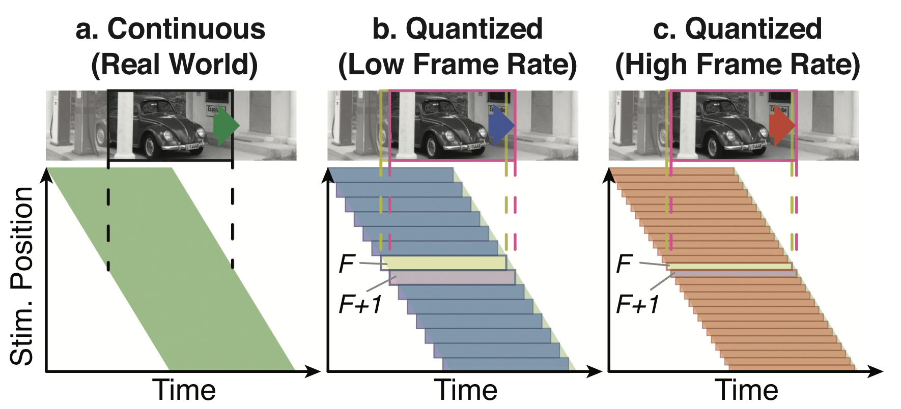
Judder is widespread in modern display systems but not when looking at real-life objects, chiefly due to static presentation: That is, a display presents us with a quickly changing series of still frames. When images are updated at the traditionally used frequency (known as frame rate, historically set at 24 unique frames per second for cinema), there often remains a perceptible residual difference between a real-life object and its displayed counterpart (see Figure 1). When frame rates are increased, judder is reduced or even becomes imperceptible to viewers.

Although judder can be seen as undesirable if one aims to reproduce reality exactly, some audiences have become accustomed to a certain look when consuming cinematic content, including the 24 frame-per-second (FPS) presentation format. This appearance is strongly associated with artistic presentation, Hollywood or other higher-budget production, and professional quality. When the frame rate is increased, some viewers balk at the smooth motion, which is then perceived as an artifact itself [Giardina 2012]. This is often referred to as the soap opera effect, associated with low-cost or home production. This reaction is generally not present when considering non-cinematic forms of entertainment [Wilcox et al. 2015]. In sports, video games and low-budget productions, high frame rates have become standard and judder is expected to be minimized. Further, a dichotomy between users that prefer smooth motion and others who prefer a certain level of “cinematic” judder exists: When considering cinematic content, we see that judder is a unique artifact that we may want to preserve, within some threshold—not too high so as to not ruin the quality of the content but not too low or we risk making viewers unhappy with the content’s new look.

An additional degree of freedom in this problem is that motion artifacts are influenced by other factors associated with the displayed content and the screen being employed by the viewer. Several factors may affect judder [Daly et al. 2015; Larimer et al. 2001], such as content brightness, dynamic range, contrast, speed and direction of motion, shutter angle and shutter speed, eccentricity in the field of view of the observer, and, of course, frame rate. Interestingly, as display technologies evolve, mainly with the introduction of high dynamic range televisions and projectors, the magnitudes of several of these factors (e.g., brightness, contrast, etc.) are changing, thus affecting their influence on judder. Feedback from artists and audiences shows that some movies that had desirable judder characteristics in a traditional cinema in the past may now appear to have too much judder when seen in high dynamic range (HDR) cinemas. This places new and restricting constraints on content creators in relation to what kind of scenes and motions can be present in their movies, effectively diminishing the HDR effect or enforcing only slow movement to be present. Our work aims to model judder perceptually, paving the way for tools that are able to quantify and control judder.

2 RELATED WORK

The differences between the natural continuous motion of an object and its discrete sampled counterpart result in perceived artifacts that we term judder. In this section, we point out that:
- Existing perceptual metrics are not sufficient to predict judder preference (Section 2.1, 2.2)
- Judder is likely to become a more prominent problem for novel display modes such as HDR (Section 2.3)
- Existing frame interpolation methods require additional information to produce perceptually pleasant results (Section 2.4)

2.1 Motion Perception

Motion perception has been widely studied [Nishida 2011], from the basics such as Fourier motion and the aperture problem to more advanced topics such as transparent motion [Mulligan and others 1992], motion aftereffects [Derrington and Badcock 1985], and biological motion [Johansson 1973]. Other vision science work directed to distortions of practical interest include the motion sharpening effect, whereby blur levels of static frames are substantially less visible when the frames are displayed in motion [Bex et al. 1995; Takeuchi and De 2005; Westerink and Teunissen 1995]. The smoothness of sampled motion without specifically referring to the common term, judder, has been investigated including the effects of intermittent occlusion [Scherzer and Ekroll 2009], which can be applied to projector shutter designs.

Perceptual image difference metrics such as HDR-VDP [Mantiuk et al. 2011] compare two images by employing a pipeline modeling the human visual system. Video difference metrics are much less common. Work from Watson and Malo on the Standard Spatial Observer [Watson and Malo 2002] contains a video quality metric based on their existing model but does not provide implementation strategies. [aydin2010video] extend their previous work on HDR image comparison to videos by employing a spatiotemporal contrast sensitivity function (STCSF) and a three-dimensional cortex transform. The window of visibility [Watson 2013; Watson and others 1986] has been developed to model the interactions of the visual system with spatiotemporal aliasing distortions due to frame rate designs and more recently this work has been extended to a pyramid of visibility by showing that the STCSF is well approximated as a linearly separable function of its factors, including the log of adapting luminance [Watson and Ahumada 2016].

Most of these works have been geared toward threshold detection of temporal artifacts as modeled by the STCSF. By contrast, our work focuses on suprathreshold appearance and aims to provide a practical model that can be used to predict and compare distortions relevant to display applications.

2.2 Judder and Frame Rate

Subjective preference for higher frame rates was studied by [Wilcox et al. 2015], who showed that in an experimental setting audiences preferred high frame rate clips to traditional 24Hz presentation. This work was later extended [Allison et al. 2016] to specifically target expert viewers with similar outcomes. A stronger preference for high frame rate presentation was found for action clips. Shutter angle was not found to play an effect on participants’ choices. Although higher frame rates were preferred, the stimuli employed in the experiments were relatively simple short clips and may not fully evoke a cinematic sensation associated with high production value feature films, which may have reduced the propensity of the audience to be disturbed by the “soap opera effect.”

Explorations specifically on the perception of judder include qualitative work on understanding what underlies the “film look” [Roberts 2002], including factors such as frame rate, object motion, and whole-frame motion (panning), as well as the causes within the eye as opposed to on-screen. The perception of double edges and their relation to source image sharpness is discussed.

Initial work on judder from a vision science perspective [Larimer et al. 2001] found that judder increases at both the high speeds (as expected), as well as the very low speeds. This result was confirmed in this work, as seen in Section 5 and 6. An initial investigation on fundamental judder perception [Daly et al. 2015] from a quantitative approach discussed four underlying components of judder: motion blur, non-smooth motion, multiple edges, and flickering. The relative weights of these distortions into an overall perception of judder are unknown, and individual variability is possible. The dominant effect was frame rate, followed by speed, but other factors had measurable effects. The study sampled few variations in a large set of perceptual factors to achieve a high level understanding of the space, and thus is not suitable as the basis of a visual model.

2.3 Display Technology

Although standard cinema specifications only require a luminance of 48cd/m2 [DCI 2012], high dynamic range and ultra-bright displays are becoming ever more common and important as part of UHD television [Nilsson 2015]. Major TV manufacturers including LG, Sony, Panasonic, Samsung, and TCL have released consumer-level HDR screens with peak luminance varying from 800 to 4000cd/m2, with yet brighter displays announced or demonstrated. With the introduction of OLED televisions into the market, ultra-high contrast display has also become ubiquitous.

Recent art has seen the effect of extended luminance and contrast explored for other perceptual factors such as color [Kim et al. 2009] and stereopsis [Didyk et al. 2012], and researchers have noted that judder is likely to become a more prominent problem for novel display modes such as HDR [McCarthy 2016; Noland 2016], confirmed by this work. Feedback from industry professionals shows that a commonly used technique to combat judder introduced by increased brightness in novel displays consists of simply reducing content brightness during grading, which is undesirable.

In the context of limited transmission bandwidth, perceived quality tradeoffs between spatial and temporal resolutions have been shown to have a nonlinear relationship [Debattista et al. 2018].

2.4 Frame Interpolation

This work is done within the context of presentation on a modern display. Such displays are generally capable of showing images at a higher rate than the traditional 24Hz (e.g., 60, 120, or 144Hz). In this section, we discuss the problem of video frame rate re-sampling. These algorithms are occasionally concerned with the removal or preservation of judder, but lack the psychophysical data to make informed editing decisions.

There is a great variety of frame interpolation methods available. Traditional methods use motion flow vectors computed during video encoding [Zhai et al. 2005], derivatives of optical flow [Mahajan et al. 2009] or even phase-based motion estimation [Meyer et al. 2015]. Because motion estimation often fails, especially when the movement is non-translational or when objects are not rigid, these methods may generate artifacts. Recent advances in machine learning have been applied to frame interpolation, both as a tool to compute better flow [Dosovitskiy et al. 2015], to generate entirely new frames at the cost of adding blur [Vondrick et al. 2016], or combine both techniques [Liu et al. 2017]. While these methods can be used to obtain video at different frame rates, they do not solve the problem of finding a desirable judder pattern intrinsically.

Templin and colleagues developed a method to simulate arbitrary frame rates on displays with high refresh rates [Templin et al. 2016]. This method is meant for fine-tuned control of frame rate effects and was developed specifically to control judder but does not provide a definite answer for what the desirable characteristics of a video asset are in terms of judder or how to predict or match judder across different display technologies. This is precisely the goal of our work.

3 EXPERIMENTAL SETUP

To study judder through psychophysical trials, an experimental setup consisting of a display capable of reliably showing content at a large range of frame rates is necessary. To test the suitability of a display for our study, we measured its refresh rate and stability with a pair of Thorlabs PDA36A photo sensors that measure light in the visible wavelengths (350–780nm) at a frequency of up to 10MHz connected to an oscilloscope. A sample measurement can be seen in the supplementary material. To assess potential crosstalk between consecutive frames, the display was filmed with a high-speed camera while displaying temporal calibration targets.

After some experimentation, we found that our LCD displays were unable to show individual frames correctly at 120Hz due to slow rise times, resulting in incorrect frame brightness. Instead, our setup consists of an LG C7 2017 55” RGBW OLED TV. The display was calibrated to a standard CIE D65 (x = 0.3127, y = 0.329) whitepoint using a Photo Research SpectraScan PR740 spectroradiometer perpendicular to the center point of the screen. The display operated at a resolution of 1920×1080.

We also found that typical video players are unable to reliably play at 120Hz without frame drops or repeats. To fix this we employed a custom OpenGL GPU implementation with multithreaded image loading from disk. To read uncompressed video frames, our application required a fast hard drive: For our resolution, 1920 ∗ 1080 ∗ 3 (RGB) ∗1 byte (8-bit images) ∗120Hz ≃ 750 MB/s, assuming a perfect system. Our server had a RAID-0 disk array providing >2GB/s read speeds and a Quadro M4000 GPU and was connected to the display via an HDMI 2.0 cable.

4 PSYCHOPHYSICAL EXPERIMENTS

Based on previous work discussed in Section 2.2 and feedback from industry content creators, we identified the main components of video that are believed to impact judder. Our goal is to examine these factors and generate a predictive model. We ran three psychophysical experiments measuring perceived judder.

4.1 Perceptual Factors Affecting Judder

The following are expected to be the strongest and most useful elements, present in all three studies:

Frame Rate. Expected to be the main factor affecting judder [Watson 2013], frame rate is in many ways the most malleable dimension for the manipulation of cinematic content as changes can be made without significantly altering the composition. Our experiments were performed on subsets of 24, 30, 60, and 120Hz. Frame rates under 24Hz are not widely employed in practice. In the practical cinematic scenarios targeted in this work [Fujine et al. 2007], rates over 120Hz are unlikely to exhibit judder, although motion artifacts could be visible at higher frame rates under different conditions, such as very high stimulus speed [Watson and others 1986].

Speed. As this work is mostly concerned with camera pans, we chose to parametrize this dimension based on panning speed, i.e., we assume the analyzed scene will have a unique dominant motion component. To select meaningful values, we turn to existing rules of thumb for pans in cinema [Burum 2007]. In many cases, a 7s pan across the screen is considered the fast limit for a traditional shot to avoid motion artifacts. We chose to probe pans with speeds of 5, 7, 11, and 17s so we have information above, at, and below this limit. These speeds translate to approximately 2, 3, 4.7, and 6.6 deg/s based on the viewing distance of three picture heights, which corresponds to a horizontal 33◦ viewing angle for the whole screen. We expect higher speeds to translate into more perceived judder. For very slow speeds, the opposite may happen due to spatial position accuracy, especially at lower spatial resolutions [Larimer et al. 2001]. These values are all within the region of smooth pursuit tracking [Li et al. 2010; Meyer et al. 1985]. Smooth pursuit has a gain slip of about 0.9, and for wide field of view, catch-up saccades are used by the visual system to continue with smooth pursuit tracking. We expect that both smooth pursuit eye movements and occasional catch-up saccades may occur for some viewers, but that the rating assessment would be accumulated during the smooth pursuit behavior during any given trial. In particular, any visibility during a saccade will be substantially suppressed.

Adapting Luminance. Known to influence spatiotemporal contrast sensitivity [Lange 1958; Van and Bouman 1967], adapting luminance has been modelled in image engineering [Barten 1989; Daly 1992]. Following common practice in this field, we model adaptation luminance as the mean of the image’s luminance in cd/m2. We expect sensitivity to rise as luminance increases, so it is reasonable to expect that judder may become more noticeable. We test mean luminance levels of 2.5, 10, and 40cd/m2. Note that image brightness varies based on scene content and the values presented here are taken as representative averages of mean luminance present in cinema and home theater for the first and second, while the final value is equally spaced but higher and represents a hypothetical high-luminance screen.

Additional factors are explored in some of our experiments:

Contrast. The STCSF operates on contrast, which is expected to be a factor. In this work, we used Michelson contrast, defined as (Imax − Imin )/(Imax + Imin ) to describe this factor, where I is the luminance image being used. Higher contrast is expected to lead to more perceived judder. We probed contrast values of 0.95, 0.75, and 0.5. Cinematic content traditionally strives to use as much of the available contrast as possible, and as such reducing contrast is usually not a feasible form of judder control.

Shutter Angle. More generally, motion blur reduces the retinal-image contrast of high spatial frequencies, potentially reducing judder. Shutter angles are traditionally described in degrees of arc with 360◦ representing a shutter that is open for the entire duration between frame captures. Smaller values represent fractional exposures: A 180◦ shutter means the sensor is exposed for half the available time. We explored shutter angle values of 360◦, 180◦, and 0◦ (the latter taken by convention when using an unaltered still image to simulate a camera pan). Blur is often used to control judder by content creators when no other options are available, but blurring strongly alters the scene leading to lost information.

Motion Direction. Previous research on judder [Daly et al. 2015] hypothesized that horizontal motions may produce more judder than vertical for some stimuli due to the better performance of horizontal smooth pursuit over vertical [Ke et al. 2013], but no data are provided to compare these results quantitatively.

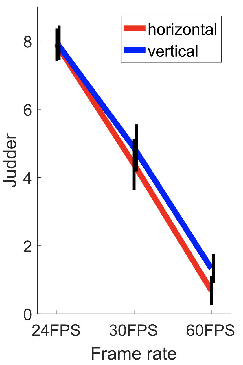
To gauge whether directionality of motion is an integral part of judder perception, we ran a brief user study. The experimental procedure, stimulus, and analysis were identical to Experiment 1 described in Section 4.2 and 5, but the only variables were frame rate at 24, 30, and 60 FPS and directionality, with the edge moving top-to-bottom (vertical) or left-to-right (horizontal). Thirteen users participated, with results shown in Figure 2. Frame rate was a significant factor (F = 410.58, p ≪ 0.01). Direction was not found to be significant (F = 2.24, p = 0.14) with horizontal and vertical showing very similar behavior in terms of judder. In the rest of this work, we focus on horizontal movement, as this is the most common case in cinema and television.

4.2 Experimental Procedure

Participants were seated comfortably in a dark room. A chin rest was not employed as we felt that simulating natural viewing conditions would be more important than restricting head movements.
The experiment was performed with binocular viewing and natural pupil size. The display was placed at a standard three picture heights from the participants [Poynton 2012].

As the goal of this work is to generate a transducer function from a high-dimentional space of parameters to judder, direct comparisons between conditions would have resulted in a prohibitively large number of trials. Instead, participants were instructed to rate stimuli in terms of judder on a scale of 0–9 (the former meaning no judder), with judder defined to participants as the absence of smooth motion. Stimuli were shown in three blocks of equal luminance (at mean luminance levels of 2.5, 10, or 40cd/m2) to allow participants to perform at a stable luminance adaptation state, with random block order and random presentation order of stimuli within each block for each participant. To allow the users to calibrate their responses to the dataset, a training session was conducted prior to each experiment that consisted of one of these three blocks chosen at random. Training results were excluded from further analysis. Results for each participant were normalized to use the entire 0–9 range to account for
user variability.

Participants could observe each stimulus as many times as necessary to make their decision, after which responses were recorded using a standard keyboard. Each run consisted of 3 frame rates, 3 luminance levels, 4 speeds, and 1 additional parameter per experiment with 3 states, totaling 108 stimuli for the main experiment and an additional 36 for the training session. Participants took, on average, 30 minutes to complete the experiment, which was judged to be the longest period possible before fatigue.

4.3 Stimuli

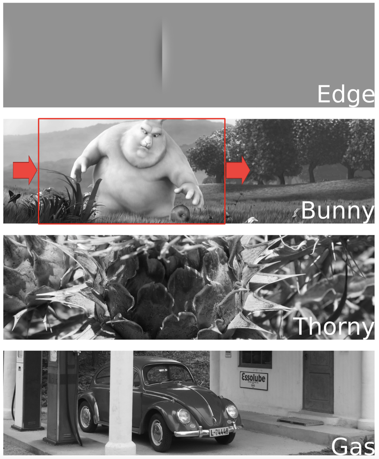
As we expect higher spatio-temporal sensitivity to achromatic stimuli [Kelly 1983], images were presented in grayscale (see Figure 3).

Experiment 1. This experiment had the following variables:

• Framerate=[30,60,120]Hz
• Mean luminance=[2.5,10,40]cd/m2
• Speed=[17,11,7,5]secondpanacrossthescreen
• MichelsonContrast=[0.5,0.75,0.95]
  We employed a traditional vision science stimulus termed “disembodied moving edge” [Savoy and Burns 1989] on a gray background. The edge moved across the screen left-to-right with the desired speed. The edge consisted of two vertical, adjacent columns of pixels with values M and m symmetric about the mean and calculated to match the desired contrast (see Appendix A), which then smoothly decayed toward the mean away from the edge.

Experiment 2. This experiment had the following variables:
- Framerate=[30,60,120]Hz
- Mean luminance=[2.5,10,40]cd/m2
- Speed=[17,11,7,5]secondpanacrossthescreen
- Images=[bunny,thorny,дas]

In this experiment, we chose to employ still image pans to provide participants with more realistic stimuli. A 1920×1080 window of a larger image is displayed and pans across the screen at the desired speed. Three images were selected, depicting a rendered scene from Big Buck Bunny1 and two natural scenes showing a thorny cactus flower with strong diagonal features and a gas station with strong vertical lines.

Experiment 3. This experiment had the following variables:
- Framerate=[24,30,60]Hz
- Mean luminance=[2.5,10,40]cd/m2
- Speed=[17,11,7,5]secondpanacrossthescreen
- Shutter Angle = [0◦, 180◦, 360◦]

In this experiment, we used only the thorny image from Experiment 2 but were interested in exploring the effect of shutter angle on judder. As the original content is a still image, we consider its shutter angle to be 0◦ by convention. Knowing the speed and frame duration for each stimulus, we computationally simulated shutter angles of 180◦ and 360◦ to see if photorealistic motion blur values (i.e., as would have been shot with a real-life camera) for image pans could be used as a viable strategy to mitigate judder. Although stronger blurring is possible and often employed as a tool in production, we chose not to include it in this test as it would significantly alter the scene. In addition, we explored lower frame rates introducing 24Hz and removing 120Hz from the set.

5 EXPERIMENT RESULTS

The results of experiments 1 to 3 were analyzed using linear mixed regression, treating participants as random effects to capture differences in their baseline rates of judder detection. The resulting p-values are reported below. Effect sizes are discussed in Section A.2.

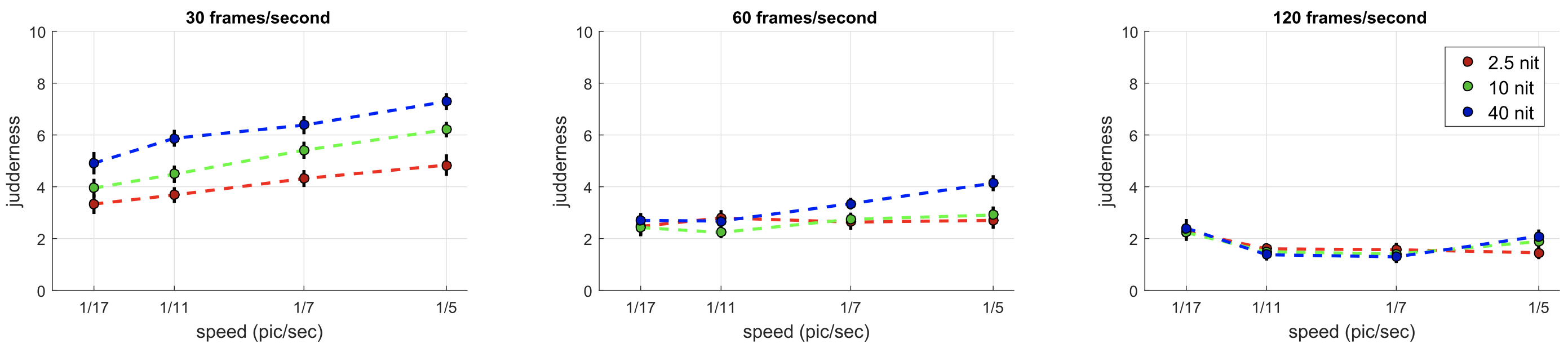
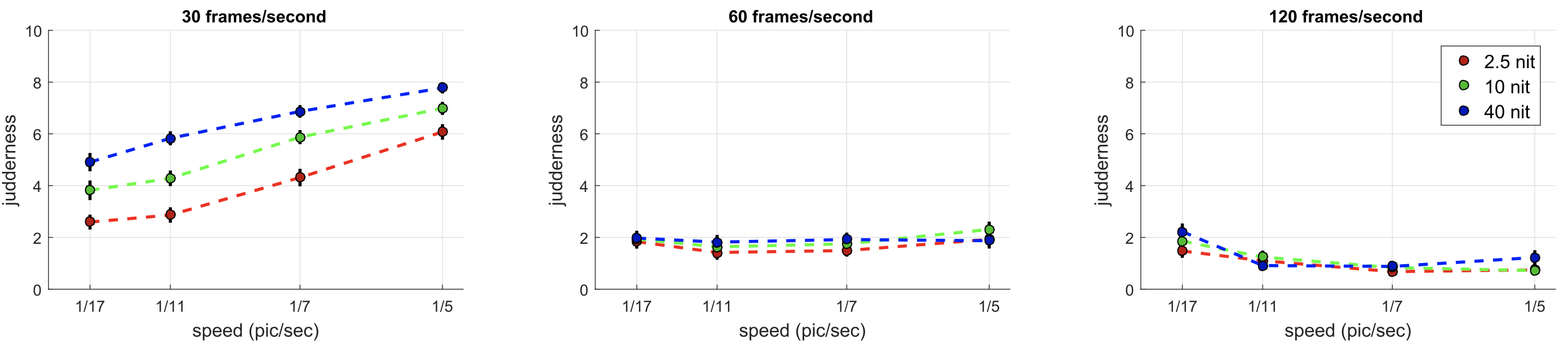
Experiment 1. Twelve participants took part. As expected from Section 4.1, significant factors included mean luminance (F = 53.68, p ≪ 0.01), frame rate (F = 633.07, p ≪ 0.01) and speed (F = 36.34, p ≪ 0.01). Contrast was not found to be a significant factor (F = 0.54, p = 0.46), possibly due to all stimuli being of suprathreshold contrast and contrast constancy effects [Georgeson and Sullivan 1975].

The results of this experiment can be seen in Figure 4; for simplicity, the plotted data have been averaged over the contrast dimension and participants. By comparing the three plots, we note that frame rate has a powerful effect on mitigating judder, with results at 120 and 60Hz showing little perceived judder, while 30Hz stimuli were all perceived with high levels of judder. A clear trend from the 30Hz plot is that, at this frame rate, judder increases uniformly with luminance. In addition, speed has a nearly linear effect on perceived judder.

Experiment 2. Eleven participants took part. Once again, mean luminance (F = 52.09, p ≪ 0.01), frame rate (F = 849.78, p ≪ 0.01), and speed (F = 40.26, p ≪ 0.01) were found to be significant factors. Type of image shown (F = 1.62, p = 0.20) was not significant.

The results can be seen in Figure 5, averaged out over the three different image types and participants for simplicity. The product of this experiment is similar to experiment 1, which validates our expectation that judder perception for more realistic stimuli still follows the expected trends.

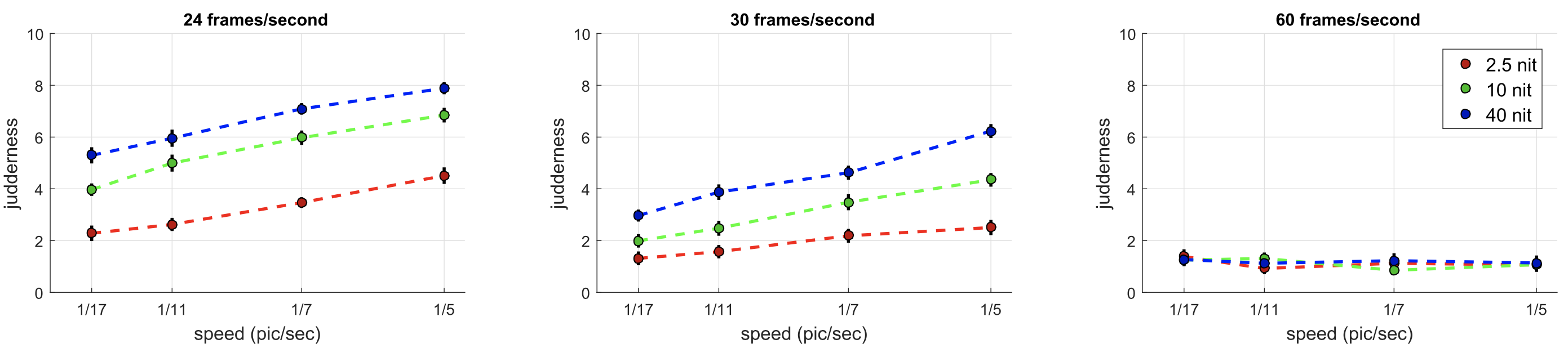
Experiment 3. Ten participants took part. Significant factors included mean luminance (F = 249.77, p ≪ 0.01), frame rate (F = 1017.50, p ≪ 0.01), and speed (F = 154.92, p ≪ 0.01). Shutter angle was not found to be a significant factor (F = 0.23, p = 0.63).

The results can be seen in Figure 6, averaged out over shutter angle and users, for simplicity. In this experiment, we introduced a lower-frame-rate condition, 24Hz, and removed the highest frame rate from previous cases, as its results contained almost no information (120Hz). As this results in a different scaling of the responses, data were normalized such that the blocks overlapping with experiments 1 and 2 have matching means before generating the model described in Section 6. Note that, as previously, little judder is experienced at 60Hz, while results for 30Hz look similar to earlier studies. At 24Hz, a stronger difference between the lowest luminance level (targeting standard dynamic range cinema) and the higher luminances is seen.

Variables that were not found to be significant were not included in our perceptual model of judder, although this result does not necessarily indicate that contrast, shutter angle, or type of image will never affect judder. It is possible, for example, that stronger distortions such as non-photorealistic blurring above 360◦ could significantly affect judder perception, but such values were not tested in this work, as they would strongly alter the look of the scene and thus do not lead to a satisfactory solution to mitigate judder.

6 JUDDER MODEL

To obtain an easily expressible model of judder ${\prosedeflabel{judder}{{J}}}$ based on the most important factors, mean luminance ${\prosedeflabel{judder}{{L}}}$ , frame rate ${\prosedeflabel{judder}{{F}}}$ , and speed ${\prosedeflabel{judder}{{S}}}$ , we combine the results of experiments 1–3 to design a single empirical model. We fit the perceptual data provided by user study participants into a second degree polynomial model:

This is an excellent fit to the psychophysical data, with a mean absolute error of 0.24 (equivalent to 9.4%) between measured and predicted judder at the probed points. To present the reader with an error metric that relates to physical quantities, we also computed the mean error in the log-luminance domain (to avoid under representing errors in low-luminance conditions). Given $N$ as the number of measured conditions, ${\prosedeflabel{error}{{O}}} (i)$ being the observed means for each condition and ${\prosedeflabel{error}{{M}}} (i)$ values predicted by our model , we calculate the error ${\prosedeflabel{error}{{E}}}$ as

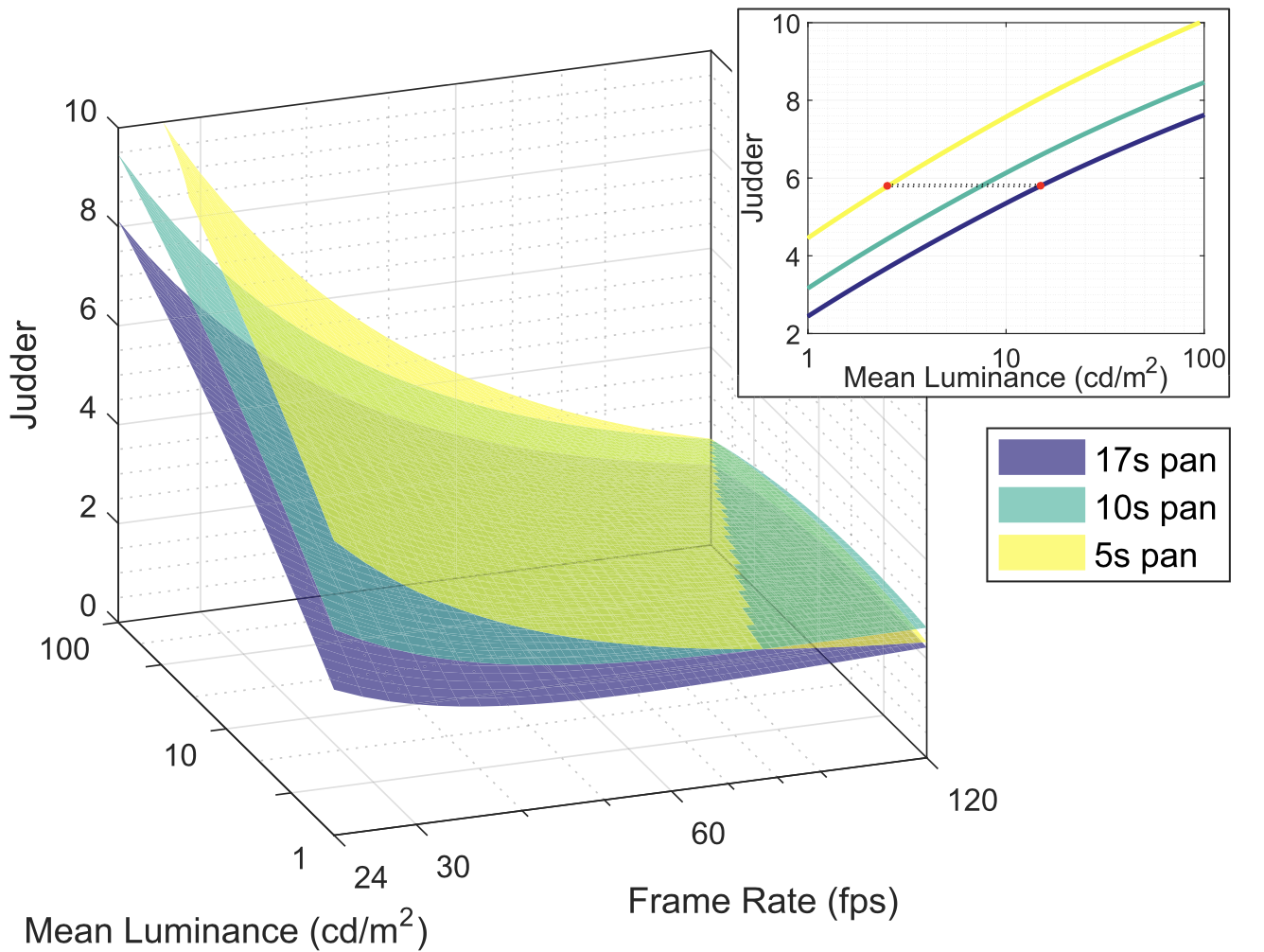
resulting in ${\proselabel{error}{{E}}}$ at approximately 1.37%. A visualization of this model for a speed of 1/7 pictures per second can be seen in Figure 7 (left). A rendering of the overlaid surfaces for various speeds and a cross section of the resulting shapes for a given frame rate can be seen in Figure 8.

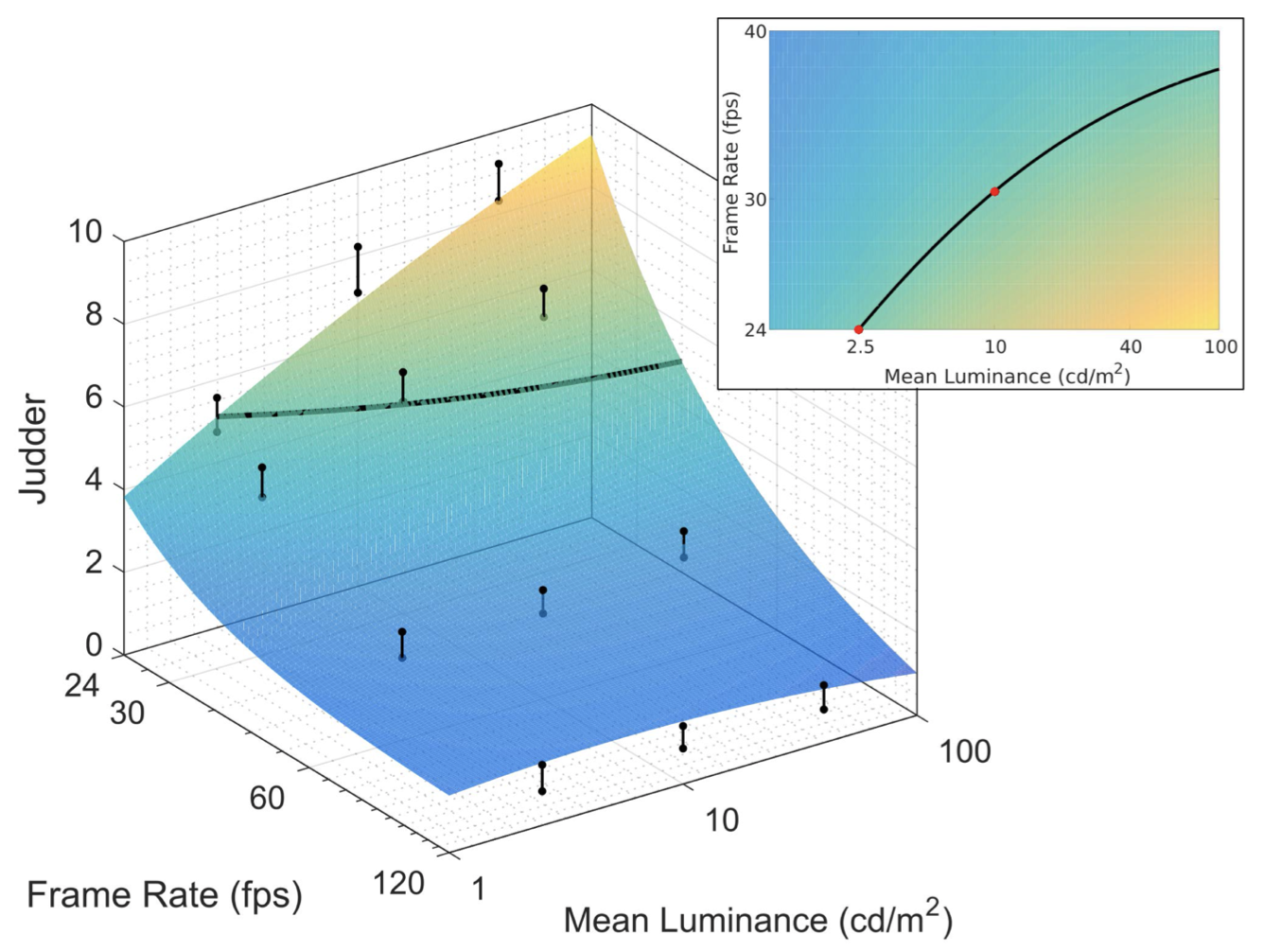
Finally, our model allows us to compute iso-lines over which perceived judder is expected to remain constant—this is a good opportunity to explore the hitherto unknown perceptual consequences of changes in judder due to different display technologies. In Figure 7 (right), we see that the predicted frame rate necessary to match the judder of a 24Hz, 2.5cd/m2 stimulus at 1/7 pic/s (a typical cinema frame rate and brightness at traditionally peak acceptable speed) displayed at 10cd/m2 is approximately 31Hz. This is significantly lower than the frame rates available in modern home theater displays. In addition, we calculate that if operating on speed, rather than frame rate, the judder of a traditionally fast 5s pan at $2.5cd/m^2$ is equivalent to that of an extremely slow 17s pan at a higher luminance of $15cd/m^2$. This further demonstrates that novel display technologies will require content creators to adapt their processes to deal with the newly introduced increase in perceptual sensitivity, as the increase in brightness will incur prohibitive judder even for slow moving objects unless frame rates are increased.

7 VALIDATION

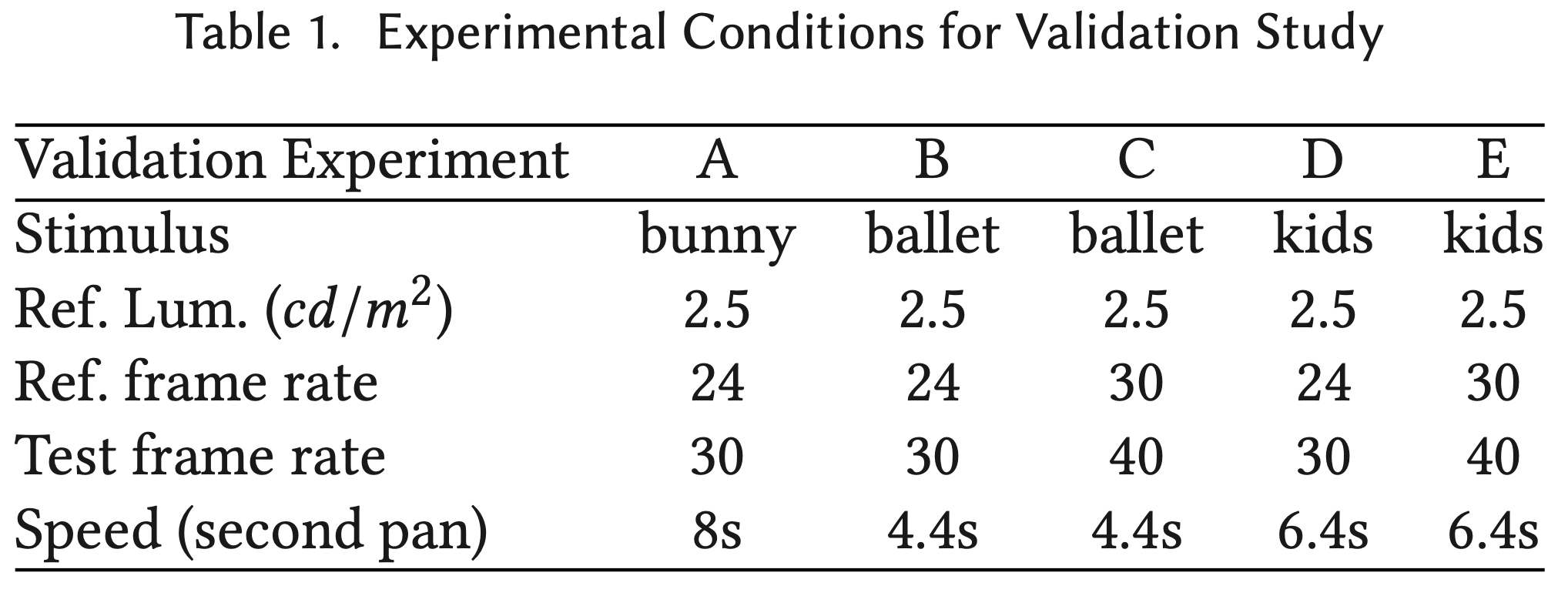
To test the validity of our model with more complex stimuli, we ran a Validation experiment. Using the same setup as the experiments described in Section 3, 15 participants were shown short reference videos at a lower frame rate and brightness. They were then presented with another version of the same video, but at a higher frame rate. The experimental task was to find the best match in terms of judder by controlling the mean luminance of the test stimulus through logmean offsets. Five stimuli were employed, two shots from Nocturne,2 dubbed Ballet and Kids, and one shot from Big Buck Bunny. All stimuli contained camera pans and were likely to generate some perceivable judder and can be seen in the accompanying video. The details for each of the five tested cases can be seen in Table 1, with additional details presented in Appendix A.4.

We computed luminance predictions to match judder between test and reference using our metric as described in Equation (1). Although no other judder metric exists, we adapted the wellknown Ferry-Porter law for flicker fusion thresholds [Tyler and Hamer 1990] to predict temporal artifact sensitivity. It is normally expressed as

where ${\prosedeflabel{judder}{{a}}}$ and ${\prosedeflabel{judder}{{b}}}$ are known constants and L is the mean luminance. If we introduce the simplifying assumption that the critical flicker fusion rate (${\prosedeflabel{judder}{{CFF}}}$) is linearly correlated through a factor ${\prosedeflabel{judder}{{M}}}$ with judder-sensitivity, then we can obtain a log-luminance equivalence like the one queried in this experiment. Denoting ${\prosedeflabel{judder}{{F_a}}}$ and ${\prosedeflabel{judder}{{F_b}}}$ as the two frame rates and ${\prosedeflabel{judder}{{L_a}}}$ , ${\prosedeflabel{judder}{{L_b}}}$ as the luminances :

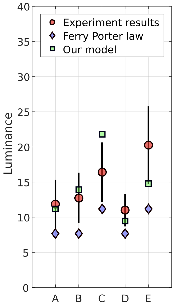
The results of this experiment can be seen in Figure 9, along with the predicted luminance match given by our model with the appropriate pan speed. Participants found the assignment to be challenging, as it included a cross-dimensional matching task across different image brightnesses. The prediction given by the static Ferry-Porter law only takes mean luminance into account and, even with the free parameter M, underestimates the luminance required to match our stimuli in every case: Using Equation (2) we obtain a mean luminance error of 17.1%. Our model achieves a mean error of 6.51%, improving the prediction in every case and falling within the 95% confidence interval in all but one case.

7.1 Applications to Content Creation

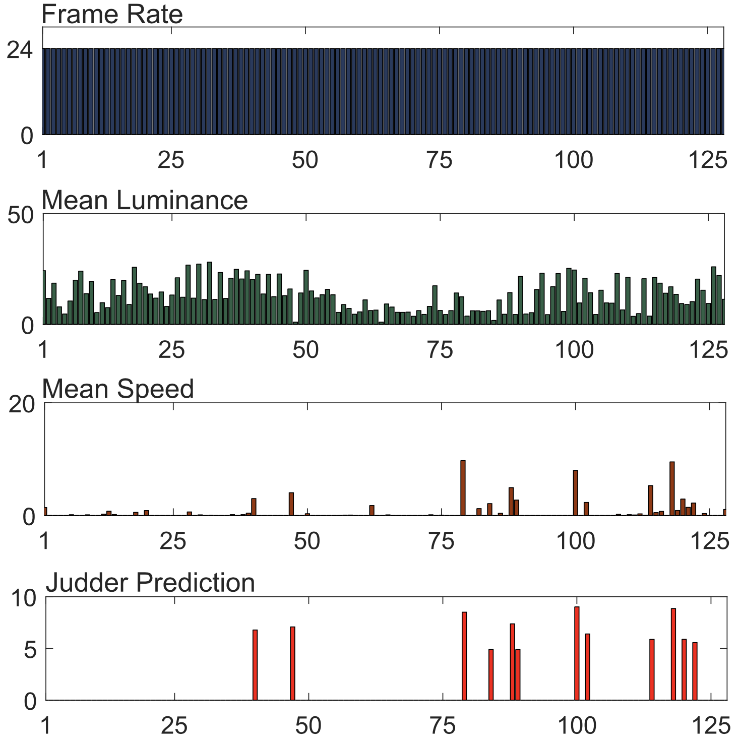
An application of our model is flagging content that is likely to produce high levels of judder in post production. Given the content and a target display, a shot boundary detector is applied to segment the video into shots. We recover the frame rate of the video and, for each shot, we calculate the mean luminance and translation speed. We proceed to apply our model as presented in Section 6. We demonstrate this technique by applying our model to the entire Big Buck Bunny short, which is composed of 128 shots. Shots that contain speed values less than the minimum explored in our user studies (i.e., a 17s pan or 2 deg/s average) were excluded from the computation, and judder prediction was set to zero. In this case, we simulate a cinema projector with a maximum and minimum brightness of 50 and 0.05cd/m2, respectively, and a gamma of 2.4 with a user sitting at three picture heights from the screen. Figure 10 shows the resulting judder prediction.

Similarly to the task of users in the validation experiment described in Section 7, content flagged as having excessive judder can be tone-mapped to a lower mean luminance range automatically. As an example, we selected shot 47 of Big Buck Bunny that showed a judder value of 7.1 in Figure 10. We can adapt the 7s rule as referenced in Section 4.1 to produce an estimate of a high boundary for acceptable judder: We set speed to the eponymous 7s pan, frame rate to a standard 24Hz, and mean luminance to 2.5cd/m2. The resulting value is 5.1 on our judder scale. We proceed to fix the speed and frame rate of the selected shot, and model judder for various mean luminance levels. We find that in order for this shot to have a predicted judder of 5.1, its mean luminance must be reduced from 16 to 3.1cd/m2 or approximately 0.72 log units. The judder scale for this shot, as well as a sample image tone mapped using a simple log-luminance offset, are shown in Figure 11. A comprehensive review of modern tone mapping methods was presented by [Eilertsen et al. 2017].

8 CONCLUSIONS, LIMITATIONS, AND FUTURE WORK

We proposed the first model that predicts the magnitude of perceived judder for a given video. We gathered psychophysical data on a number of relevant factors using simple stimuli and later demonstrated that these measurements are also valid for complex scenes. Our experiments generated valuable data that can provide guidance to content creators considering emerging display technologies, such as necessary updates to existing rules of thumb in cinematography. This information can also be useful to display manufacturers and content providers when considering technical requirements for consumer technologies. Finally, perceptual judder modeling is crucial for frame rate re-sampling applications to avoid judder or other undesirable artifacts such as the “soap opera effect.”

Our work has certain limitations: The first is that our model is only valid for clips that contain relatively stable motion with a single dominant component, such as a camera pan. The “ballet” clip used in Section 7, for example, contains a speed ramp-up that may have caused our results to deviate from the data gathered from users as they may have graded on the slower or faster portion of the clip. Clips where little to no motion is detected are not expected to contain visible judder and are not supported by our model.

Extending Fourier-based spatio-temporal video difference prediction approaches (Section 2.1) to supra-treshold differences for judder would be an interesting task. Such algorithms require lengthy computation times per video, however, making them impractical for common real-time applications.

Although this work focused chiefly on judder arising from camera pans, as this is the most common scenario, an interesting avenue for future work would be to generalize the model to separate objects on the scene. User attention can be predicted using a visual saliency model and object speed could be estimated through optical flow techniques.

Our studies explored an overall sense of judder, but there are certainly different perceptual components to this artifact that contribute to the whole as subcomponents. At this stage of inquiry, we felt the strongest need would be to address the overall perception of judder. A logical next step would be to study the perceptual components of judder as their understanding may be useful to algorithm design. We hope our work encourages the community to further explore spatio-temporal artifacts and make all our experimental data fully available for analysis.

9 APPENDIX

9.1 Disembodied Edge Calculation

Given a desired Michelson contrast $c$ and mean ${\proselabel{judder}{{L_a}}}$, we calculate the maximum and minimum values $\proselabel{Edge}{M}$ and $m$ as $\proselabel{Edge}{M}= {\proselabel{judder}{{L_a}}} (1 + c)$, $m= {\proselabel{judder}{{L_a}}} (1 − c)$. As a consequence of this, the resulting Michelson contrast is exactly $( {\proselabel{judder}{{L_a}}} + {\proselabel{judder}{{L_a}}} *c − {\proselabel{judder}{{L_a}}} + {\proselabel{judder}{{L_a}}} * c)/( {\proselabel{judder}{{L_a}}} + {\proselabel{judder}{{L_a}}} * c + {\proselabel{judder}{{L_a}}} − {\proselabel{judder}{{L_a}}} * c)=2 {\proselabel{judder}{{L_a}}} *c/(2 {\proselabel{judder}{{L_a}}} )=c$. If one of these values does not fit within the dynamic range of the display being used, then both values can be shifted using a multiplier $k$ so that $\proselabel{Edge}{M}= \proselabel{Edge}{M}* k$, $m = m* k$ to accommodate these practical constraints.

The maximum and minimum values computed in the previous step are set to fall off to the background level ${\proselabel{judder}{{L_a}}}$ in a smooth fashion. In our application, we employed a screen with horizontal resolution of 1920 pixels and found a visibly acceptable smoothness to be achieved using a Gaussian falloff with standard deviation of 45 pixels.

9.2 Effect Size

Effect size can be calculated from an arbitrary scale such as the judder scale introduced by our article. We include the calculation of a Pearson’s correlation coefficient in the supplementary material containing the raw data for experiments 1–3. Following the guidelines set by “A Power Primer” (1992), we find that in all three experiments the independent variables speed and luminance had a small to medium strength effect on judder, frame rate had a strong effect, and the fourth variable (contrast, image type, and shutter angle, respectively) had an effect less than small.

9.3 Judder Model

Below, on the left, are the coefficients for our judder model as described in Section 6. On the right, the power of the appropriate term. This information is also available in the supplementary material. Note that our model takes as input speed in pixels per second on a screen with a horizontal resolution of 1,920×1,080 at three picture heights’ distance, subtending a 33◦ field of view. If a speed S is given in degrees per second, then a conversion function for speed should be used as follows: $γ({\proselabel{judder}{{S}}}) = {\proselabel{judder}{{S}}} * 1920$ . In addition:

9.4 Validation Data

To compute a judder prediction using our model for an arbitrary scene, a speed measurement is necessary. As we are mostly concerned with panning scenes we expect the clip to have a strong main motion component due to the camera motion. We computed a frame-to-frame best-fit translation, which is pooled over all frames, filtered (speeds below 1 deg/s fall short of the smooth pursuit range [Meyer et al. 1985] and are filtered out), and averaged to compute the speed. Note that this procedure is only valid for clips that contain relatively stable motion. We obtained a mean panning speed of approximately 8s for Bunny, a fast 4.4s for Ballet, and 6.4s for Kids.

10 ACKNOWLEDGMENTS

The authors thank Shane Ruggieri for helping prepare the video for the article and Sema Berkiten for final edits. We thank Shane, Thad Beier, and Jim Crenshaw for the insightful discussions on industry practices relating to judder manageulent and motion in general. We thank Thomas Wan and the immersive experience team for help with the experimental setup and hardware. We thank the user study participants for their efforts. We thank Timo Kunkel and Sema for help with style and Seth Frey for help with the statistical analysis.

11 REFERENCE