1 INTRODUCTION

Technologies for Virtual and Augmented Reality are currently experiencing a new boom. Companies such as Facebook (Surround 360), Google (Jump), Jaunt VR, GoPro (Omni), Samsung (Gear VR), Microsoft (Hololens), Magic Leap, Oculus, and many others are marketing omnidirectional camera systems and head-mounted displays. While the basic concepts underlying Virtual Reality (VR) systems have been around already for a few decades, the performance of hardware and software for capture, rendering, and display is now getting to a point where more immersive experiences are possible.

While rendered VR based on computer generated content has reached an impressive level, the capture of high-resolution, immersive stereoscopic real-world content remains challenging in practice, since it usually has to be stitched from multiple input video streams, e.g., using camera arrays. Seamless 2D stitching of such content is nowadays supported by many camera systems. However, in order to capture and display high-quality stereoscopic 3D content, many more views with larger inter-camera parallax have to be captured, and one has to convert the captured parallax into consistent, seamless stereoscopic output images.

One potential approach is image-based rendering utilizing depth information extracted from the input views (e.g., [Shum and Kang 2000]), where the stereoscopic output is generated depending on the viewer’s viewing position and direction. However, with only sparse input available as in our setting, robust and sufficiently accurate depth estimation for arbitrary scenes remains challenging, often resulting in noticeable visual artifacts.

A milestone in this context have been the works of [Peleg and Ben-Ezra 1999, Peleg et al. 2001], which demonstrated how view-direction independent images can be generated from densely captured images using a single camera rotating off-center. This insight significantly simplified the creation of panoramic stereo, since a single pair of correspondingly generated panoramic images can provide a plausible omnistereoscopic impression, i.e., a stereoscopic impression in all viewing directions on the equatorial plane. The price is that the generated images are multi-perspective, and hence do not exactly correspond to a real-world, view-direction dependent stereo geometry that is identical to human stereo perception.

A key advantage of their omnistereoscopic representation in the context of VR is that only a small modification to the stitching process allows for changes of the virtual viewpoint position, enabling a more natural interaction and immersive experience of the VR content compared to static stereoscopic images. However, in practice, existing high-resolution omnistereo approaches (e.g., [Richardt et al. 2013]) require a very large number of input views, in the order of several tens to hundreds, to generate convincing virtual head motion effects. Building a corresponding video camera array is a difficult practical challenge.

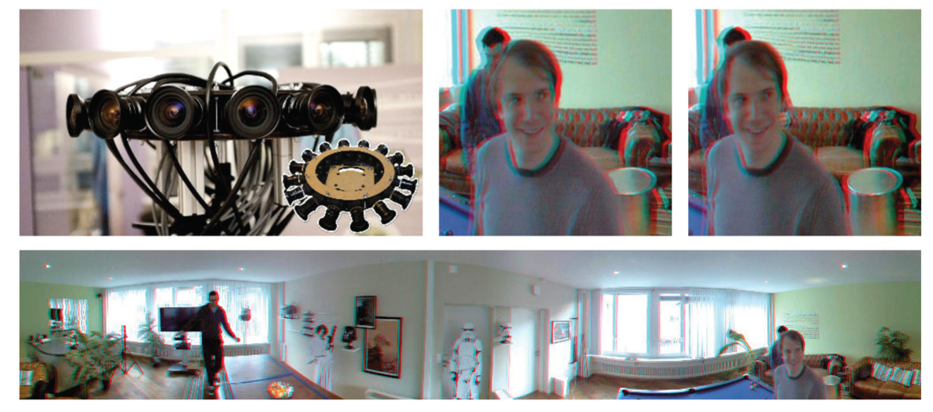
In this article, we describe a complete and practicable pipeline for the capture and display of real-world VR video content. In particular, we try to address important questions that have remained open in previous works. On the practical side, we discuss a solution that allows the generation of plausible stereo panoramas, including virtual head motion, from a small number of input videos. Our prototype is a camera array consisting of only 16 machine vision cameras (see Figure 1). On the theoretical side, we provide an analysis that relates stereoscopic output parallax and the available virtual head motion to the camera array geometry, which is an important prerequisite in order to be able to capture convincing, immersive real-world VR. We further discuss additional tools such as multi-perspective projection in order to mix real-world VR with computer generated content.

We show several real-world video panoramas that are suitable for real-time stereoscopic viewing with support for virtual head-motion, e.g., using an Oculus or Google Cardboard HMD. We compare to alternative solutions such as image-based rendering using depth, and to the Facebook Surround 360 system. In addition, we discuss and simulate alternative array and camera designs that, we hope, provide a useful guide for other researchers for building omnistereo video capture systems.

2 RELATED WORK

2D panoramas of a scene are traditionally obtained by stitching multiple pictures sharing a common single center of projection, e.g., acquired by a purely rotating perspective camera [Brown and Lowe 2007; Hartley and Zisserman 2003; Kopf et al. 2007]. See the extensive survey by [Szeliski 2006] for more details. 2D panoramic stitching tools are now commonly available on consumer cameras and smartphones. Similar tools and products also exist for video panoramas, where multiple cameras with overlapping field of view capture the scene, such as the Point Grey Ladybug camera, the FlyCam, or the PanaCast camera. The issue with such camera arrays is that, in order to create seamless 2D output panoramas, one has to hide or compensate for the parallax between the individual input views, which can, for example, be achieved by image warping [Jia and Tang 2008; Kang et al. 2004; Lee et al. 2016; Perazzi et al. 2015; Shum and Szeliski 2000] or seam-optimization [Efros and Freeman 2001; Zhang and Liu 2014]. See, e.g., [Perazzi et al. 2015] for a more detailed overview of 2D approaches.

In contrast to 2D panoramas, for the creation of stereoscopic panoramas, parallax between input views is desired, i.e., the scene has to be observed from different viewpoints. One solution is to rotate a pair of stereo cameras [Couture et al. 2011; Zhang and Liu 2015] or a lightfield camera [Birklbauer and Bimber 2014] and then stitch the acquired pictures. These approaches provide limited stereo due to the short camera baseline, and are challenging to extend to omnidirectional stereoscopic video acquisition for dynamic scenes as required for VR applications. [Hedman et al. 2017] capture images from a moving camera, and then perform textured 3D mesh reconstruction that can be used for view synthesis. While this allows a wider stereo effect, it is also limited to static scenes. Another alternative is pushbroom imaging, which has been extensively applied and studied in the context of satellite images [Gupta and Hartley 1997] and for linear acquisition, e.g., of facades [Agarwala et al. 2006; Kopf et al. 2010; Rav-Acha et al. 2008; Román and Lensch 2006; Zheng et al. 2011]. Such approaches still do not support dynamic scenes and 360 omnidirectional stereo.

To overcome these limitations, it was proposed to rotate a camera off-center [Ishiguro et al. 1992]; Peleg and Ben-Ezra 1999; Peleg et al. 2001; Richardt et al. 2013; Shum and He 1999]. Stereoscopic panoramic images can then be created by selecting appropriate columns from the input images. A key aspect of these approaches is that the resulting stereo panoramas are omnidirectional, i.e., a single pair of panoramic images generated with these approaches provides a plausible stereo impression in all viewing directions on the equatorial plane. While the resulting images are multiperspective and, hence, are not equivalent to the view-direction dependent result of, e.g., a regular stereo camera pair, the resulting stereo is still visually convincing (see [Seitz and Kim 2002] for a detailed discussion). An important advantage in the context of our work is that such a view-direction independent solution is much more feasible in the context of real-time VR applications, because a single pair of images can be used to provide stereo in all viewing directions on the equatorial plane, leading to significantly reduced computational overhead and storage requirements [Shum et al. 2005; Simon et al. 2004]. Recently it has been shown that omnistereoscopic panoramas can be created using as few as three extreme wide angle lenses [Chapdelaine-Couture and Roy 2013] or only two 360 spherical cameras [Matzen et al. 2017]. However, this is at the price of considerably reduced effective output resolution. A second major advantage of this omnidirectional representation is that it rather easily supports changes in perspective, corresponding to a virtual head motion of the viewer, without the need for more complex image-based rendering techniques requiring an accurate depth representation [Shum and Kang 2000].

A remaining limitation of the above approaches is, however, that video results of dynamic real-world scenes are challenging to create in practice. The main reason for this limitation is that all above approaches require a comparatively large number of input views to capture a sufficiently dense lightfield of the scene, which makes it impossible to capture dynamic content data with an array of cameras. A few companies have recently announced commercial solutions based on camera rigs similar to ours (e.g., Facebook Surround 360, Google Jump, Jaunt VR). While the Google Jump algorithm is described in [Anderson et al. 2016], the underlying methods are proprietary and not accessible. Only Facebook Surround 360 provides publicly available source code. In the experiments section, we provide qualitative comparisons to the Facebook system.

In summary, we describe in detail how a sparse camera rig can be used in order to create high-quality omnistereo, including support for virtual head motion and fully dynamic scenes, making capture and VR display of real-world scenes possible. In addition, we discuss all necessary system parameters in order to gain full control over the resulting output stereo, which is essential for creating immersive virtual experiences.

3 OVERVIEW

First, we will describe how to process the input views coming from a sparse omnidirectional camera array in order to create the dense representation required for synthesizing omnistereoscopic panoramas with support for virtual head motion. We discuss how to parameterize and interpolate the captured light rays using pure image-domain operations, so that, despite the sparse input, no accurate scene information (such as depth) is required.

In the second main section, we then provide a detailed analysis of various aspects of this pipeline, ranging from expected stereoscopic output parallax to the range of virtual head motion that is feasible for a particular array design. We provide derivations for ray tracing and projection of computer generated content directly into the multiperspective output panoramas, and discuss various additional aspects relevant for using the proposed pipeline in practical VR applications.

4 PANORAMA CREATION FROM SPARSE INPUT

4.1 Camera Setup and Parameterization

We consider a sparse camera array composed of $n$ cameras covering a complete 360-degree field of view; see Figure 1. In a preprocess, we estimate the camera calibration parameters (extrinsic and intrinsic) with standard calibration techniques [Zhang 2000] and bundle adjustment, and then radially undistort the images.

In an ideal setup, the cameras lie on a circle of radius ${\prosedeflabel{pipeline}{{r}}}$ , and the camera intrinsic calibration matrix can be written

where ${\prosedeflabel{pipeline}{{f_x}}}$ and ${\prosedeflabel{pipeline}{{f_y}}}$ denote the focal length in pixels in the horizontal and vertical directions , and $( {\prosedeflabel{pipeline}{{c_x}}} , {\prosedeflabel{pipeline}{{c_y}}} )$ the principal point [Hartley and Zisserman 2003]. Noting ${\prosedeflabel{pipeline}{{α}}}$ the angle of the camera along the circle , the pose of each camera is defined as

The corresponding camera projection matrix that maps 3D world coordinates to pixel coordinates is

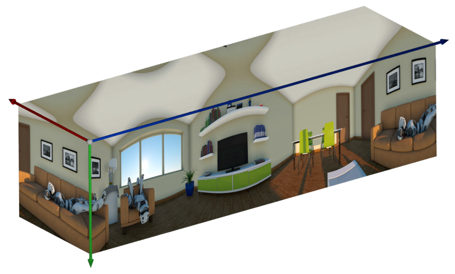
We then define the dense lightfield for a single point in time as $L ( {\proselabel{pipeline}{{α}}} , {\proselabel{pipeline}{{x}}}, {\proselabel{pipeline}{{y}}})$, which we have to reconstruct from the sparse camera input (see Figure 2 for an example of a synthetic scene). The value at a location $( {\proselabel{pipeline}{{α}}} , {\proselabel{pipeline}{{x}}}, {\proselabel{pipeline}{{y}}})$ corresponds to the measured irradiance along the ray

$$ {\proselabel{pipeline}{{R}}} ^T( {\proselabel{pipeline}{{α}}} )(\lambda \cdot {\proselabel{pipeline}{{K}}} ^{-1}( {\proselabel{pipeline}{{x}}}, {\proselabel{pipeline}{{y}}},1)^T - {\proselabel{pipeline}{{\textbf{t}}}} )\tag{4}\label{4}$$

where $ λ > 0$ represents the position along the ray.

4.2 Lightfield Reconstruction

Our aim is to reconstruct $ L ( {\proselabel{pipeline}{{α}}} , {\proselabel{pipeline}{{x}}} , {\proselabel{pipeline}{{y}}} )$ from a sparse set of input views $\hat{I}_i$ with $i =1,...,n$.The first step is to map the captured input images into the coordinate frame of $L$ by associating each input image $\hat{I}_i$ with a camera angle ${\proselabel{pipeline}{{α_i}}}$ using the estimated camera calibration. In order to approximate the ideal camera setup described in the previous section, where all cameras reside on a circle, we align each
input image $\hat{I}_i$ with the expected input at angle ${\proselabel{pipeline}{{α_i}}}$ by applying the corresponding homography. Referring to the thus transformed images as $I_i$, we now have

$$L ( {\proselabel{pipeline}{{α}}} _i, {\proselabel{pipeline}{{x}}} , {\proselabel{pipeline}{{y}}} ) \approx I _i ( {\proselabel{pipeline}{{x}}} , {\proselabel{pipeline}{{y}}} )\tag{5}\label{5}$$

Then, the problem of reconstructing $L$ comes down to performing an accurate view interpolation in ${\proselabel{pipeline}{{α}}}$. For an accurate image space approach, it is important to understand how a given 3D point ${\proselabel{pipeline}{{X}}}$ moves in $({\proselabel{pipeline}{{x}}},{\proselabel{pipeline}{{y}}})$ when varying the camera angle ${\proselabel{pipeline}{{α}}}$.

Trajectories of Scene Points in Image Space. Rather than considering the projection of a fixed 3D point when rotating the camera about the origin $o$ by some angle ${\proselabel{pipeline}{{α}}}$, changing the point of view can provide a more intuitive understanding: by keeping the camera fixed and rotating the 3D point with the inverse rotation instead, the same trajectory can be obtained. The path can thus be interpreted as observing a 3D point that travels along a cylindrical surface.

Assuming that the depth at a given location ${\proselabel{pipeline}{{\textbf{x}}}}= ({\proselabel{pipeline}{{x}}},{\proselabel{pipeline}{{y}}})^⊤$ is known, the nonlinear path in image space can be reconstructed by backprojecting according to Equation (4), rotating the resulting 3D point ${\proselabel{pipeline}{{X}}}$, and finally projecting it with Equation (3). When representing the 3D point ${\proselabel{pipeline}{{X}}}$ in cylindrical coordinates, its change in position is linear in the angle ${\proselabel{pipeline}{{α}}}$. Let the map ${\prosedeflabel{pipeline}{{φ_d}}} : {\proselabel{pipeline}{{R}}}^2 → {\proselabel{pipeline}{{R}}}^2$ denote the backprojection onto a cylinder with radius $d$ followed by a conversion to cylindrical coordinates . Then, knowing two corresponding image points ${\prosedeflabel{pipeline}{{x_i}}}$ and ${\prosedeflabel{pipeline}{{x_j}}}$ measured at angles ${\prosedeflabel{pipeline}{{α_i}}}$ and ${\prosedeflabel{pipeline}{{α_j}}}$ and their radial depth $d$ w.r.t . to the origin $o$ allows to define the nonlinear path in image space

in terms of a linear interpolation in the transformed space. Here, we assume that ${\proselabel{pipeline}{{α_i}}} < {\proselabel{pipeline}{{α}}} < {\proselabel{pipeline}{{α_j}}}$ such that the weight ${\proselabel{pipeline}{{t}}}({\proselabel{pipeline}{{α}}})$ is given by

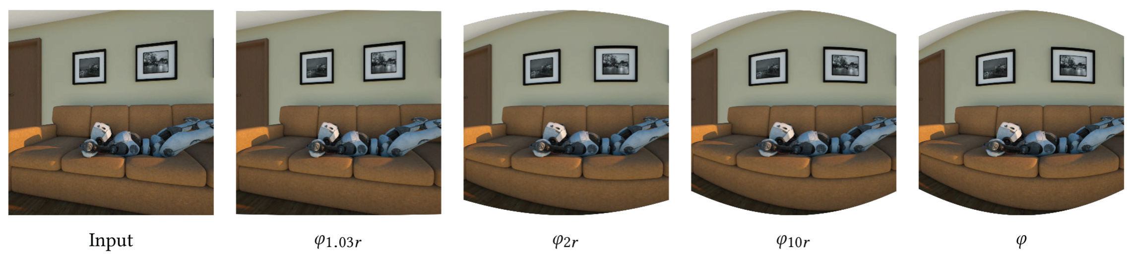
Although ${\proselabel{pipeline}{{φ_d}}}$ does allow using image space correspondences for an accurate view interpolation, it still depends on the depth of the scene point as it determines the radius of the cylinder. However, Figure 3 illustrates that the transformation an image undergoes is almost constant when varying the cylinder radius from around $2{\proselabel{pipeline}{{r}}}$ to ∞. This indicates that trajectories of points can be well approximated by using a very large cylinder radius, even when they are relatively close. By letting $d → ∞$, one can express the mapping in a depth independent way as

with

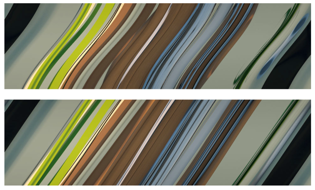
Figure 4 depicts ${\proselabel{pipeline}{{α}}}-{\proselabel{pipeline}{{x}}}$-slices of $L({\proselabel{pipeline}{{α}}}, {\proselabel{pipeline}{{x}}}, {\proselabel{pipeline}{{y}}})$ before and after transformation with ${\proselabel{pipeline}{{φ}}}$. Curved lines become straightened after the transformation, which indicates that linear interpolation indeed is an appropriate approximation to the point trajectory. Due to this insight, we are now able to compute intermediate views based on image space correspondences as follows.

Computing Intermediate Views. As a preprocessing step, we first compute forward and backward flows between all consecutive image pairs. To this end, we slightly adapt a commonly available method [Brox et al. 2004] and minimize the energy

$$\begin{align*} E(u_{ij}) = \int_{\Omega} \Psi(|I_i({\proselabel{pipeline}{{x}}})-I_j(H_{ij}({\proselabel{pipeline}{{x}}}+u_{ij}({\proselabel{pipeline}{{x}}})))|^2) \,dx \\ + {\proselabel{pipeline}{{γ}}}\int_{\Omega} \Psi(|\nabla I_i({\proselabel{pipeline}{{x}}})-\nabla I_j(H_{ij}({\proselabel{pipeline}{{x}}}+u_{ij}({\proselabel{pipeline}{{x}}})))|^2) \,dx \\ + β \int_{\Omega} \Psi(|Ju_{ij}({\proselabel{pipeline}{{x}}})|^2) \,dx \end{align*} \tag{10}\label{10}$$

As it is commonly done, we use a robust penalization function $Ψ({\proselabel{pipeline}{{s}}}^2)=\sqrt{{\proselabel{pipeline}{{s}}}^2+ε^2}$, where $ε=10^{−3}$ is a small constant and $J$ denotes the Jacobian. However, instead of directly computing correspondences between the original input images $I_i$ and $I_j$, we propose to leverage the cameras intrinsic and extrinsic calibration information to guide the flow estimation. To achieve this, we effectively preregister $I_j$ to $I_i$ using the homography induced by the plane at infinity $H_{ij} = {\proselabel{pipeline}{{K}}}_jR_{ij}{\proselabel{pipeline}{{K}}}_i^{−1}$ [Hartley and Zisserman 2003]. Incorporating the homographyi $H_{ij}$ into the minimization problem allows for a better initialization since accounting for the camera intrinsics and the relative rotation between the cameras allows to bring all objects into closer alignment in image space. In fact, distant objects can already be well aligned by this homography such that the correspondence estimation problem now mostly comes down to refining initial matches on closer objects. Since optical flow estimation is a non-convex problem, having a better initialization is important as it makes it less likely to get stuck in local minima. Besides yielding a better initialization, incorporating the homography into the minimization problem offers an additional advantage: since a homography can describe a nonlinear mapping in image space, it can account for some of the linear and nonlinear parts of the overall correspondence field between the original input images $I_i$ and $I_j$ , which otherwise may be hard to reconstruct with a first order smoothness term that pushes the correspondence field to be piecewise constant.

Initially, we anticipated a temporal consistency term in the flow estimation would be required to tackle temporal flickering. However, in practice, we observed that the results obtained by our independently computed flows are temporally sufficiently consistent (see supplementary video). The same observation has also been made by [Perazzi et al. 2015] for monoscopic panoramic video stitching.

Following the findings of the previous section, we now use these correspondences to synthesize intermediate views. When given a camera angle ${\proselabel{pipeline}{{α}}} ∈ [0, 2π )$, we can find the two closest input images, which are related to the cameras capturing views at the angles ${\proselabel{pipeline}{{α_i}}}$ and ${\proselabel{pipeline}{{α_j}}}$, respectively. Then, we compute the warp fields

$$ \begin{align*} w_{ij} = {\proselabel{pipeline}{{φ}}}^{−1}((1-{\proselabel{pipeline}{{t}}}({\proselabel{pipeline}{{α}}}))·{\proselabel{pipeline}{{φ}}}+{\proselabel{pipeline}{{t}}}({\proselabel{pipeline}{{α}}})·({\proselabel{pipeline}{{φ}}}◦H_{ij}◦(id+u_{ij}))) \\ w_{ji} = {\proselabel{pipeline}{{φ}}}^{−1}({\proselabel{pipeline}{{t}}}({\proselabel{pipeline}{{α}}})·{\proselabel{pipeline}{{φ}}}+(1−{\proselabel{pipeline}{{t}}}({\proselabel{pipeline}{{α}}}))·({\proselabel{pipeline}{{φ}}}◦H_{ji}◦(id+u_{ji}))) \end{align*} \tag{11}\label{11}$$

and synthesize the novel view from angle ${\proselabel{pipeline}{{α}}}$ as

$$ L({\proselabel{pipeline}{{α}}},{\proselabel{pipeline}{{x}}},{\proselabel{pipeline}{{y}}})=(1−{\proselabel{pipeline}{{t}}}({\proselabel{pipeline}{{α}}}))·I^{w_{ij}}_i({\proselabel{pipeline}{{x}}})+{\proselabel{pipeline}{{t}}}({\proselabel{pipeline}{{α}}})·I^{w_{ji}}_j({\proselabel{pipeline}{{x}}}) \tag{12}\label{12}$$

where $I_i^{w_{ij}}$ corresponds to $I_i$ forward-warped using $w_{ij}$ . A single panoramic image can then be obtained by fixing ${\proselabel{pipeline}{{x}}}$, i.e., a particular image column, to obtain an ${\proselabel{pipeline}{{α}}}$-${\proselabel{pipeline}{{y}}}$ slice of $L$(see Figure 2). Correspondingly, a stereoscopic output panorama can be created by picking two ${\proselabel{pipeline}{{α}}}$-${\proselabel{pipeline}{{y}}}$ slices at different column positions ${\proselabel{pipeline}{{x}}}$.

Usually, it is desirable to have square pixels in the output panorama. Therefore, we determine the sampling rate in α such that the pixel width in the output panorama matches the pixel height in the input image. The pixel height in the input image corresponds to $1/ {\proselabel{pipeline}{{f_y}}} $ when considering an image plane at distance 1. With $n$ samples, the pixel size in the output panorama is $2π/n$. Thus, we use $n = 2π {\proselabel{pipeline}{{f_y}}}$ samples in ${\proselabel{pipeline}{{α}}}$ when aiming for square pixels.

This concludes the explanation of our interpolation method. Not only the choice of the method, but also the choice of the interpolation points is important. In this scenario, the choice of interpolation points corresponds to the camera setup, which we detail on next.

5 ANALYSIS AND PRACTICAL GUIDELINES

In order to create perceptually plausible stereoscopic video, e.g., for VR applications using head-mounted displays, it is essential to have full control over the output parameters such as parallax, stereoscopic disparity, or the possible amount of virtual viewpoint changes in the panoramic output images.

We, therefore, first have to understand the image formation model, i.e., how 3D points are projected into a panorama. Knowing this, we can measure the role of different parameters of the capture system such as the number of cameras $n$, the circle radius ${\proselabel{pipeline}{{r}}}$, and the focal lengths ${\proselabel{pipeline}{{f_x}}}$ and ${\proselabel{pipeline}{{f_y}}}$ , on a given panorama.

5.1 Panoramic Image Formation

When fixing ${\proselabel{pipeline}{{α}}}$, the projection of Equation (3) allows to project a world point $\DeclareMathOperator*{\argmax}{arg\,max} \DeclareMathOperator*{\argmin}{arg\,min} \begin{align*} \idlabel{ {"onclick":"event.stopPropagation(); onClickSymbol(this, '$\\\\textbf{X}$', 'pipeline', 'def', false, '')", "id":"pipeline-$\\\\textbf{X}$", "sym":"$\\\\textbf{X}$", "func":"pipeline", "localFunc":"", "type":"def", "case":"equation"} }{ {\textbf{X}} } & = {\begin{pmatrix} \idlabel{ {"onclick":"event.stopPropagation(); onClickSymbol(this, 'X', 'pipeline', 'use', false, '')", "id":"pipeline-X", "sym":"X", "func":"pipeline", "localFunc":"", "type":"use", "case":"equation"} }{ {\mathit{X}} }\\\idlabel{ {"onclick":"event.stopPropagation(); onClickSymbol(this, 'Y', 'pipeline', 'use', false, '')", "id":"pipeline-Y", "sym":"Y", "func":"pipeline", "localFunc":"", "type":"use", "case":"equation"} }{ {\mathit{Y}} }\\\idlabel{ {"onclick":"event.stopPropagation(); onClickSymbol(this, 'Z', 'pipeline', 'use', false, '')", "id":"pipeline-Z", "sym":"Z", "func":"pipeline", "localFunc":"", "type":"use", "case":"equation"} }{ {\mathit{Z}} }\end{pmatrix}}^T\\\eqlabel{ {"onclick":"event.stopPropagation(); onClickEq(this, 'pipeline', ['Y', 'X', 'Z', '$\\\\textbf{X}$'], false, [], [], 'YCRcdGV4dGJme1h9JGAgPSAoWCxZLFopXlQ=');"} }{} \end{align*} $ by

$$\begin{pmatrix} {\proselabel{pipeline}{{x}}}\\{\proselabel{pipeline}{{y}}} \end{pmatrix} ≅ {\proselabel{pipeline}{{K}}}({\proselabel{pipeline}{{R}}}({\proselabel{pipeline}{{α}}}) {\proselabel{pipeline}{{\textbf{X}}}} + {\proselabel{pipeline}{{\textbf{t}}}} ) \tag{13}\label{13}$$

where $({\proselabel{pipeline}{{x}}}, {\proselabel{pipeline}{{y}}})$ is the projection in inhomogenous coordinates (by the operator ≅). Since a panorama is just a $( {\proselabel{pipeline}{{α}}} ,{\proselabel{pipeline}{{y}}})$ slice of $L$ obtained by fixing ${\proselabel{pipeline}{{x}}}$, the panoramic camera model can be obtained by fixing ${\proselabel{pipeline}{{x}}}$ instead of ${\proselabel{pipeline}{{α}}}$ and solving for $( {\proselabel{pipeline}{{α}}} ,{\proselabel{pipeline}{{y}}})$. This leads to an equation of the form (see details in the Appendix)

$${\proselabel{pipeline}{{A}}} sin({\proselabel{pipeline}{{α}}} ) + {\proselabel{pipeline}{{B}}} cos({\proselabel{pipeline}{{α}}} ) = {\proselabel{pipeline}{{C}}}\tag{14}\label{14}$$

with coefficients

Two solutions exist:

up to 2π, where $\DeclareMathOperator*{\argmax}{arg\,max} \DeclareMathOperator*{\argmin}{arg\,min} \begin{align*} \idlabel{ {"onclick":"event.stopPropagation(); onClickSymbol(this, 'ϕ', 'pipeline', 'def', false, '')", "id":"pipeline-ϕ", "sym":"ϕ", "func":"pipeline", "localFunc":"", "type":"def", "case":"equation"} }{ {\mathit{ϕ}} } & = arcsin\left( \frac{\idlabel{ {"onclick":"event.stopPropagation(); onClickSymbol(this, 'C', 'pipeline', 'use', false, '')", "id":"pipeline-C", "sym":"C", "func":"pipeline", "localFunc":"", "type":"use", "case":"equation"} }{ {\mathit{C}} }}{\idlabel{ {"onclick":"event.stopPropagation(); onClickSymbol(this, 'D', 'pipeline', 'use', false, '')", "id":"pipeline-D", "sym":"D", "func":"pipeline", "localFunc":"", "type":"use", "case":"equation"} }{ {\mathit{D}} }} \right)\\\eqlabel{ {"onclick":"event.stopPropagation(); onClickEq(this, 'pipeline', ['D', 'C', 'ϕ'], false, [], [], 'z5UgPSBhcmNzaW4oQy9EKQ==');"} }{} \end{align*} $ , $\DeclareMathOperator*{\argmax}{arg\,max} \DeclareMathOperator*{\argmin}{arg\,min} \begin{align*} \idlabel{ {"onclick":"event.stopPropagation(); onClickSymbol(this, 'D', 'pipeline', 'def', false, '')", "id":"pipeline-D", "sym":"D", "func":"pipeline", "localFunc":"", "type":"def", "case":"equation"} }{ {\mathit{D}} } & = \sqrt{{\idlabel{ {"onclick":"event.stopPropagation(); onClickSymbol(this, 'A', 'pipeline', 'use', false, '')", "id":"pipeline-A", "sym":"A", "func":"pipeline", "localFunc":"", "type":"use", "case":"equation"} }{ {\mathit{A}} }}^{2} + {\idlabel{ {"onclick":"event.stopPropagation(); onClickSymbol(this, 'B', 'pipeline', 'use', false, '')", "id":"pipeline-B", "sym":"B", "func":"pipeline", "localFunc":"", "type":"use", "case":"equation"} }{ {\mathit{B}} }}^{2}}\\\eqlabel{ {"onclick":"event.stopPropagation(); onClickEq(this, 'pipeline', ['A', 'B', 'D'], false, [], [], 'RCA9IOKImihBXjIgK0JeMik=');"} }{} \end{align*} $, and $\DeclareMathOperator*{\argmax}{arg\,max} \DeclareMathOperator*{\argmin}{arg\,min} \begin{align*} \idlabel{ {"onclick":"event.stopPropagation(); onClickSymbol(this, 'γ', 'pipeline', 'def', false, '')", "id":"pipeline-γ", "sym":"γ", "func":"pipeline", "localFunc":"", "type":"def", "case":"equation"} }{ {\mathit{γ}} } & = arctan\left( \frac{\idlabel{ {"onclick":"event.stopPropagation(); onClickSymbol(this, 'B', 'pipeline', 'use', false, '')", "id":"pipeline-B", "sym":"B", "func":"pipeline", "localFunc":"", "type":"use", "case":"equation"} }{ {\mathit{B}} }}{\idlabel{ {"onclick":"event.stopPropagation(); onClickSymbol(this, 'A', 'pipeline', 'use', false, '')", "id":"pipeline-A", "sym":"A", "func":"pipeline", "localFunc":"", "type":"use", "case":"equation"} }{ {\mathit{A}} }} \right)\\\eqlabel{ {"onclick":"event.stopPropagation(); onClickEq(this, 'pipeline', ['A', 'B', 'γ'], false, [], [], 'zrMgPSBhcmN0YW4oQi9BKQ==');"} }{} \end{align*} $. To obtain ${\proselabel{pipeline}{{α}}}$, we simply pick the solution for which ${\proselabel{pipeline}{{\textbf{X}}}}$ lies in front of the camera. Given ${\proselabel{pipeline}{{α}}}$, it is straightforward to obtain ${\proselabel{pipeline}{{y}}}$ by the projection of Equation (13).

5.2 Amount of Stereoscopic Parallax

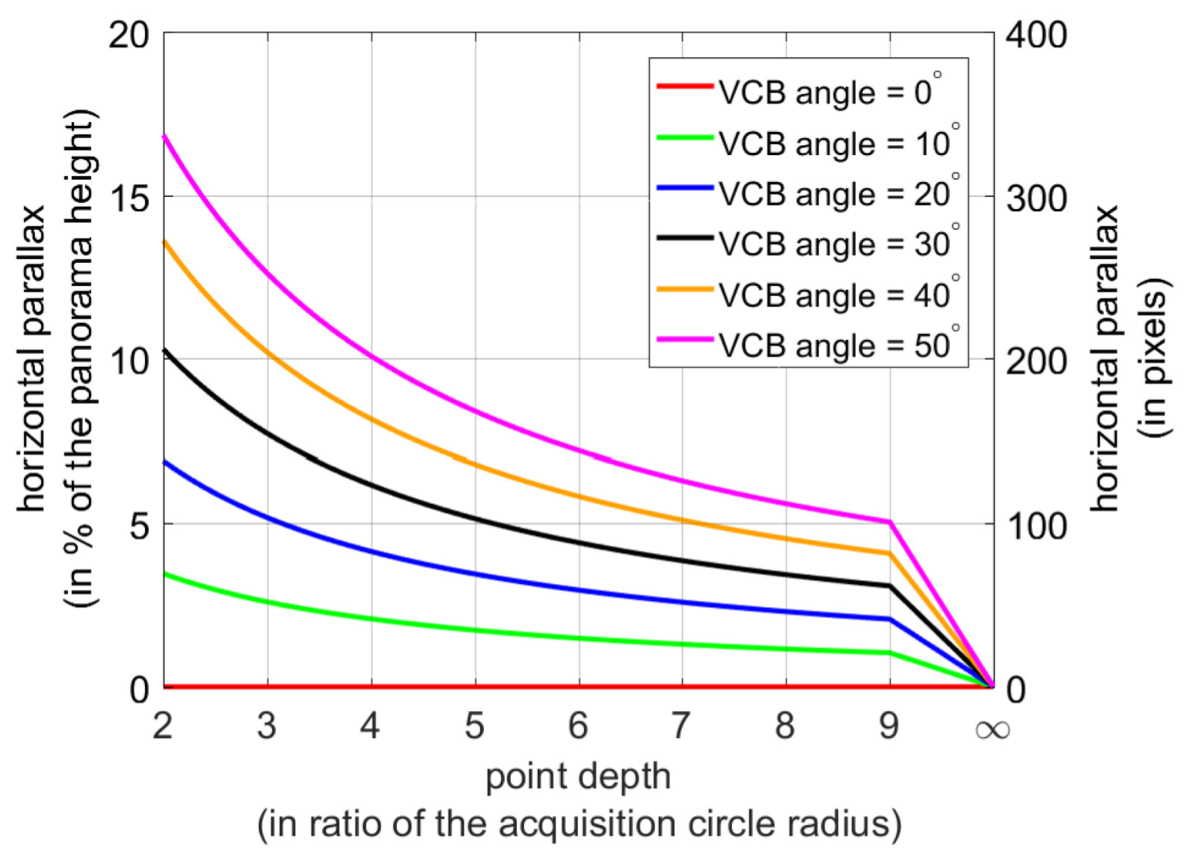
With the panoramic image formation model, we can now understand the relation between the scene depth and the parallax in the output panoramas. As explained in Section 4.2, the stereoscopic output panorama is created from two column slices. For example, the left panorama is created from the slice at column ${\proselabel{pipeline}{{x}}}_l$ , and the right panorama at column ${\proselabel{pipeline}{{x}}}_{\proselabel{pipeline}{{r}}}$ . For simplicity, in this section, we assume that all cameras in the rig have a fixed focal length $f$. Furthermore, we consider symmetric cases around the center column ${\proselabel{pipeline}{{x}}}_c$ oftheinputimages,i.e.,$|{\proselabel{pipeline}{{x}}}_l −{\proselabel{pipeline}{{x}}}_c|=|{\proselabel{pipeline}{{x}}}_{\proselabel{pipeline}{{r}}} −{\proselabel{pipeline}{{x}}}_c|$.The distance ${\proselabel{pipeline}{{x}}}_{\proselabel{pipeline}{{r}}} −{\proselabel{pipeline}{{x}}}_l$ controls the virtual camera baseline (VCB). This is analogous to the distance between a pair of cameras in a conventional stereo rig controlling the resulting stereoscopic output parallax. To conduct experiments in a way that is invariant to the input image size, we consider the VCB angle, which is given by $2 · {\proselabel{pipeline}{{ω}}} ({\proselabel{pipeline}{{x}}}_{\proselabel{pipeline}{{r}}})$ according to Equation (9).

Figure 5 verifies that the parallax in the stereoscopic output panorama decreases with larger scene depth and smaller VCB angle. Furthermore, it also shows how to choose the acquisition and synthesis parameters to match the disparity capabilities of desired output devices, such as head-mounted displays or autostereoscopic screens with a limited disparity range.

5.3 Minimum Visible Depth

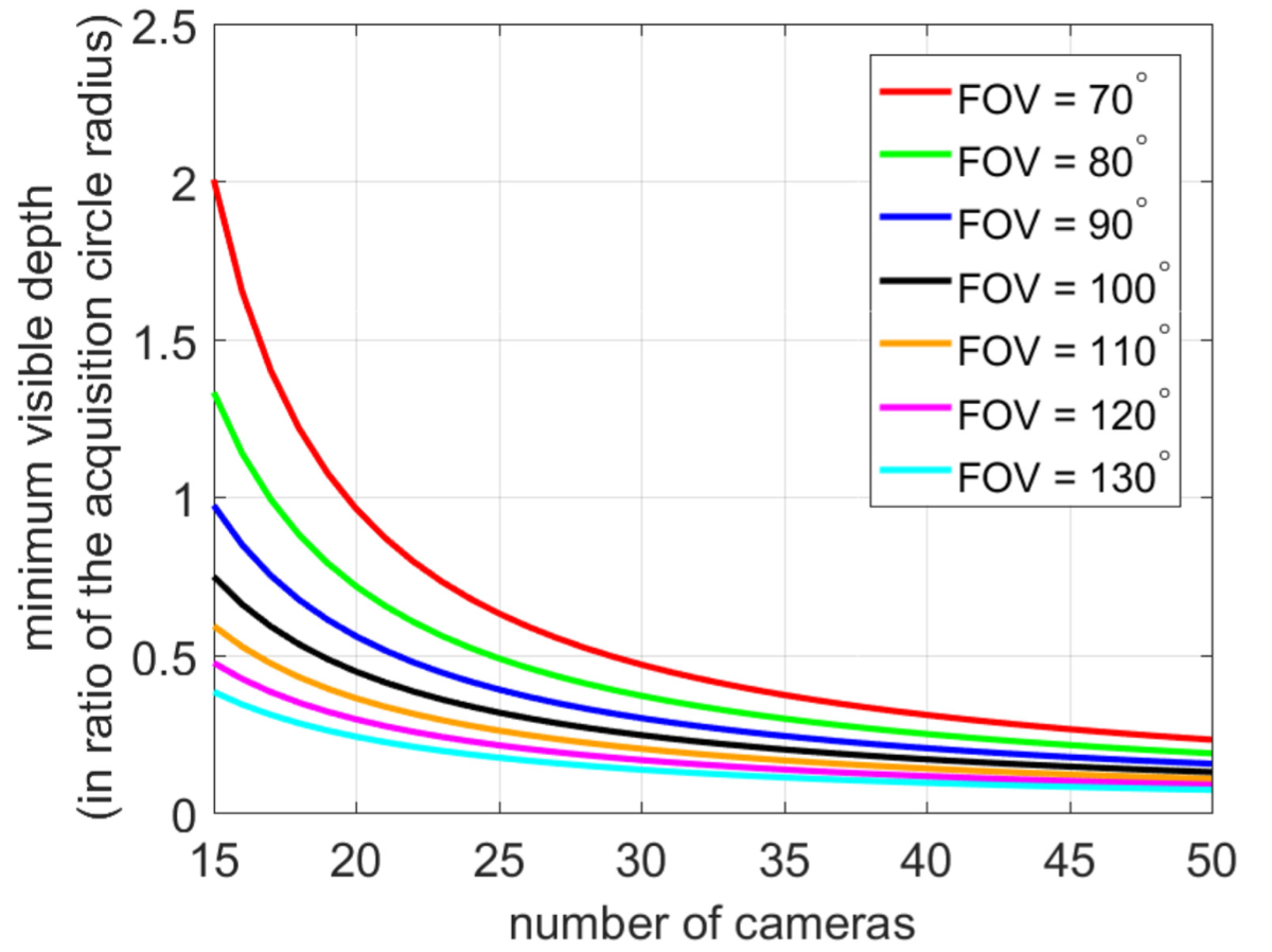
In order to capture a large amount of parallax, objects have to be sufficiently close to the camera (Section 5.2). However, due to the sparse sampling, an object too close to the camera array might be observed by only one camera, and therefore cannot be correctly interpolated. An important question that naturally arises is: what is the minimum distance that can be observed by two cameras. We derive that the minimum distance is (see details in the Appendix)

$${\proselabel{pipeline}{{r}}} \frac{\sin(π − β/2)}{\sin(β/2−θ)}\tag{17}\label{17}$$

where ${\proselabel{pipeline}{{r}}}$ is the camera circle radius, $β$ is the field of view of the camera, and $θ = 2π /n$ is the angle between two cameras (uniform distribution on the camera rig circle). Figure 6 illustrates the values of the minimum depth with respect to the number of cameras of the rig and the camera’s field of view. It shows that the minimum distance decreases with more cameras and a wider field of view.

5.4 Analysis of the Image Space View Interpolation

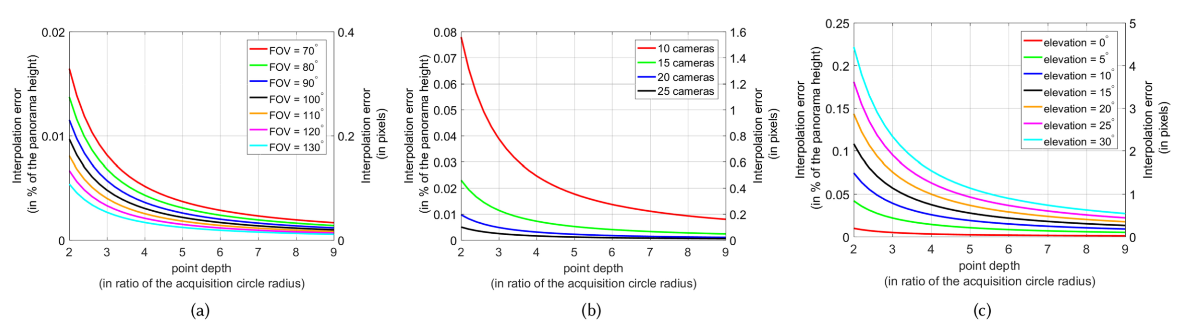
In Section 4.2 we mentioned that the trajectories of scene points can be well approximated solely by image space correspondences without knowing their actual depth. This section analyzes the approximation quality of the image space view interpolation in detail and shows that the deviation compared to a view interpolation based on scene depth is small. Our analysis covers different configurations of camera arrays as well as varying depth and elevation of world points. Here, the elevation of a world point is defined as the angle between the camera rig plane and the line connecting the world point and the camera rig center. The plots in Figure 7 show that the interpolation error is small and goes toward zero. When the world point is far away from the cameras , the field of view is wider (Figure 7(a)) and more cameras are used (Figure 7(b)).

The above experiments, in conjunction with Figure 6, indicate that it is beneficial to use a camera array composed of many cameras with a wide field of view. On the other hand, using many cameras increases the requirements in terms of data bandwidth, memory, synchronization, and processing. A wider field of view decreases the effective resolution. Concretely, this means that users need to carefully consider the tradeoff between the scene volume that can be captured and the setup requirements; or adapt the acquisition setup according to the data provided in Figures 6 and 7.

5.5 Virtual Head Motion

A particularly intriguing feature of the omnistereoscopic panorama representation is the ability to simulate virtual head motion, i.e., shifting the viewer’s location sideways within the captured scene. In practice, sideways head motion can be achieved simply by synthesizing the stereoscopic output panorama using two columns from the lightfield $L$ that are not symmetrically placed around the center column, which in turn provides a view of the scene from varying perspectives. This principle has been demonstrated, for example, in [Peleg et al. 2001]. However, in order to be applicable in real-time VR applications, e.g., using a head-tracked Oculus Rift, a user’s head motion has to be properly mapped.

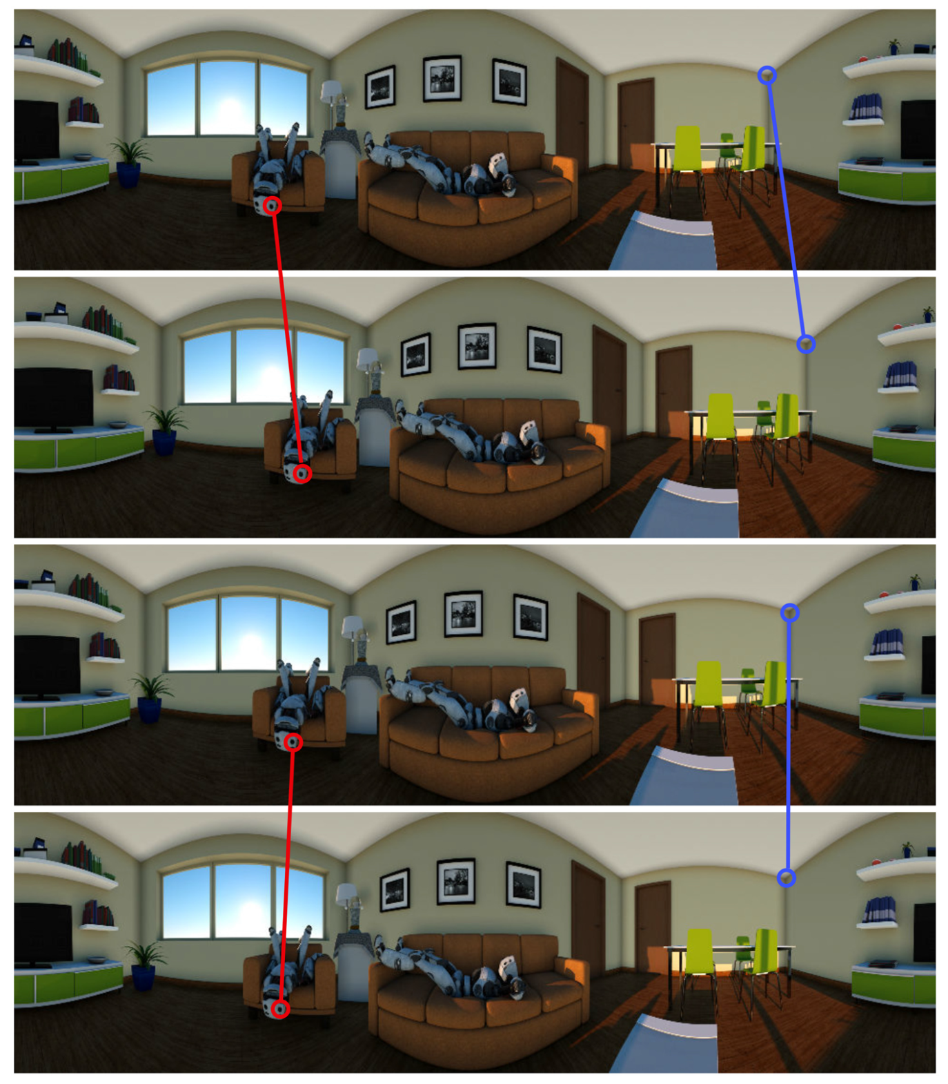
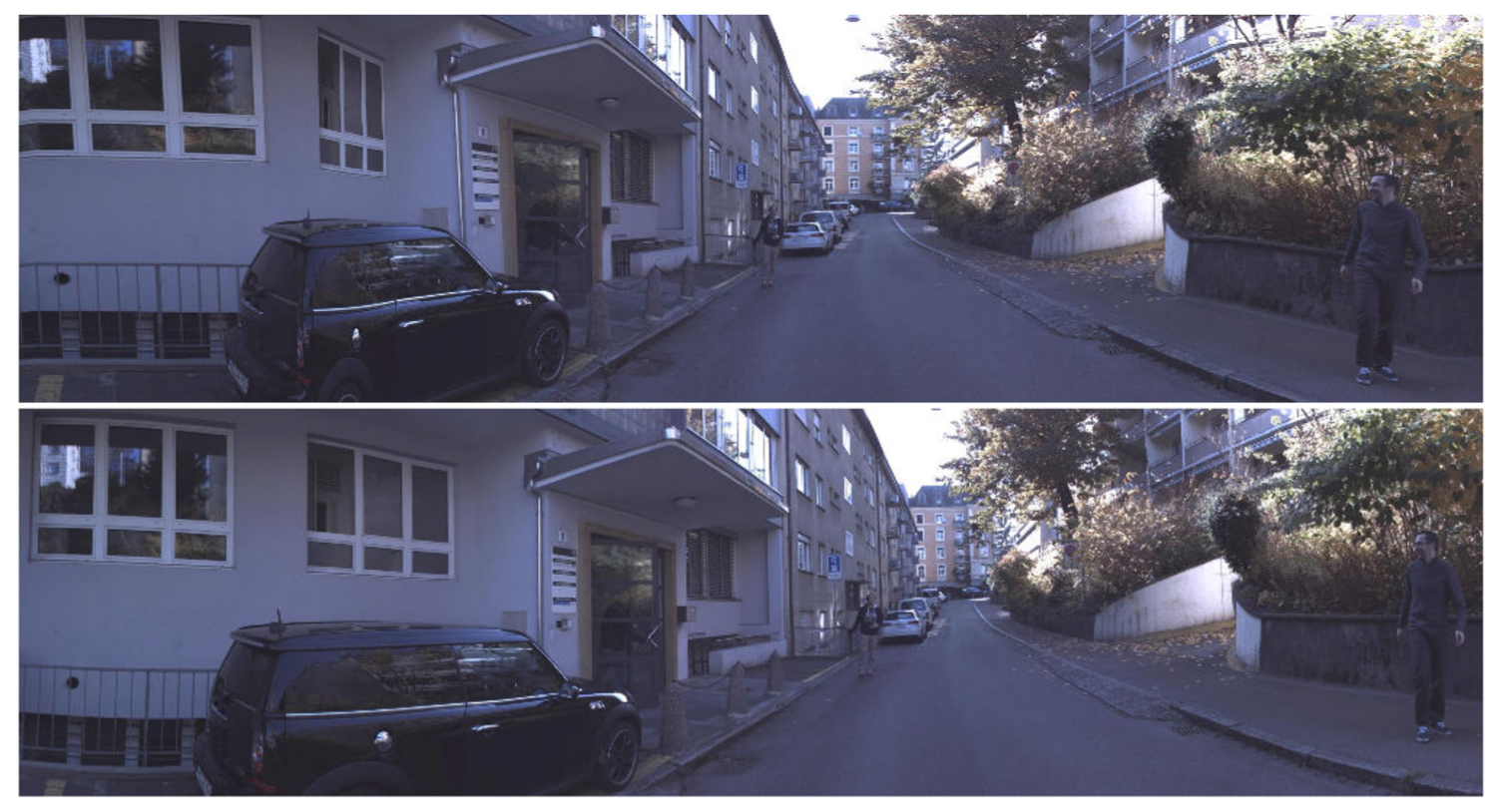
One issue is that picking a ${\proselabel{pipeline}{{α}}}$-${\proselabel{pipeline}{{y}}}$ slice from the lightfield $L$ for generating a panorama (Section 4.2) not only changes the perspective onto the scene, but also modifies the orientation of the panorama (see Figure 8). In order to synthesize proper output panoramas required for virtual head motion effects, the orientation between the panoramas must stay consistent. This means that points at infinity must be fixed in the generated panoramas, i.e., be at the same location. Let P and P′ be two panoramas generated from extracting α-y slices from L by fixing the columns x and x′, respectively. Noting α and α′, the orientation of a point at infinity in P and P′, we must then have α = α′. In practice, this can be achieved by shifting P′ by ${\proselabel{pipeline}{{ω}}}({\proselabel{pipeline}{{x}}}′) − {\proselabel{pipeline}{{ω}}}({\proselabel{pipeline}{{x}}})$ where ${\proselabel{pipeline}{{ω}}}({\proselabel{pipeline}{{x}}})$ is defined in Equation (9) (see details in the Appendix). Figure 8 illustrates the effect of fixing points at infinity on a synthetic sequence.

After this registration, a virtual head motion effect that mimics a sideways head motion can be achieved by tracking the sideways headmotion of a user and selecting the panorama based on this data. In our prototype, we typically use a subset (just 10–20) of all panoramic images as this is sufficient for creating a convincing head motion effect. These views are precomputed and then loaded by the VR viewer in real time. This approach directly transfers to the stereoscopic case where one simply selects both the left and the right panoramas based on the head position. The described approach allows for a real-time head motion effect in stereo as it comes down to selecting two appropriate panoramas. Although the head motion parallax induced by the sideways head motion is usually best observed when the user is not rotating at the same time, this is not strictly required. Our system also supports the scenario where sideways head motion and rotation occur simultaneously. Results of head motion with fixed orientation in stereo are available in the supplementary video.

6 RESULTS

In this section, we discuss results generated with our prototype array and the described processing pipeline. Please see the supplemental material for dynamic video results.

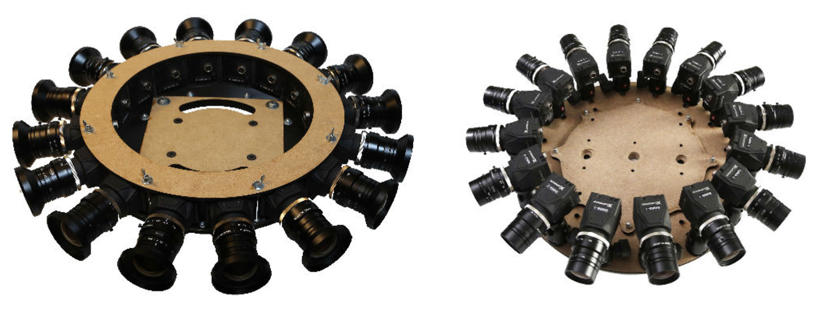
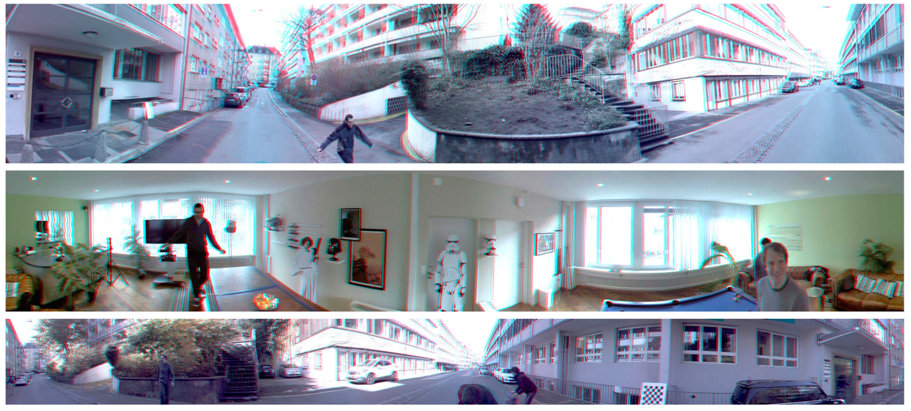
Real-World Results. We show real-world results for different scenarios including static setups where the camera rig is fixed as well as dynamic setups with a moving camera array; see Figures 1 and 13. Our experiments cover both indoor and outdoor scenes. For capture, we have used two different 360◦ camera rig prototypes. One has been assembled by hand with approximate camera placement and orientation, while the other one has been created with a 3D printer (Figure 9). Both prototypes are equipped with n = 16 synchronized cameras that are more or less uniformly distributed on a circle of radius r = 20cm and r = 15cm, respectively, with cameras pointing outward.

We used Lumenara Lt425 cameras equipped with Kowa lenses with a field of view of approximately 70◦ and 50◦, respectively, and captured videos at a resolution of 2048 × 2048 pixels per camera and 30 frames per second.

We processed the acquired videos on a standard desktop computer equipped with an Intel i7 3.2Ghz and 64GB RAM. Our current C++ prototype implementation running on CPU takes about 20 minutes per time instance in total from the reading of the n input images to the generation of all the panoramas with the complete range of column disparities, including optical flow computation, which is the current bottleneck. This is an offline preprocess that does not require any user interaction. Once the panoramas are generated, our view-independent approach allows real-time headmotion effects. We expect significant speed improvements from an optimized GPU implementation.

Necessity of Flow-based Correspondences. Figure 10 shows crops of panoramas with and without using the flow-based correspondences. The latter one is achieved by simply setting all flows ui j = 0 during panorama reconstruction. In this case, ghosting artifacts occur because homographies alone do not allow for an accurate reconstruction. Without using an accurate interpolation, creation of stereoscopic content and changes of viewpoint are not possible. In general, if the optical flow is inaccurate, artifacts may become visible in the output panorama. This is not specific to our method, but common for all flow-based techniques. Both Figures 10 and 19 can give an intuition of how our system behaves when supplied with inaccurate optical flow. Given that they constitute extreme cases and, still, the generated panoramic image is well recognizable, this shows that our system, in particular due to our pre-alignment, is designed to fail gracefully when supplied with inaccurate optical flow.

Influence of Calibration. Figure 11 illustrates the errors that occur when neglecting the camera parameters in the reconstruction process (Section 4.2). Especially for our handmade prototype, the real camera pose can considerably deviate from the theoretically expected one. In this case, the flow-based interpolation will automatically compensate for these deviations and still produce a photometrically consistent panorama, e.g., without artifacts such as ghosting. However, this comes at the cost of distorting the scene geometry. Considering the camera parameters allows to produce geometrically consistent panoramas, which is crucial for creating stereoscopic content and viewpoint animations.

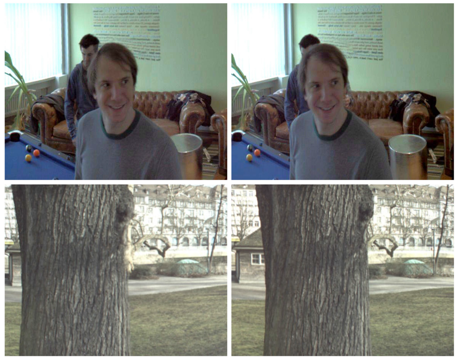
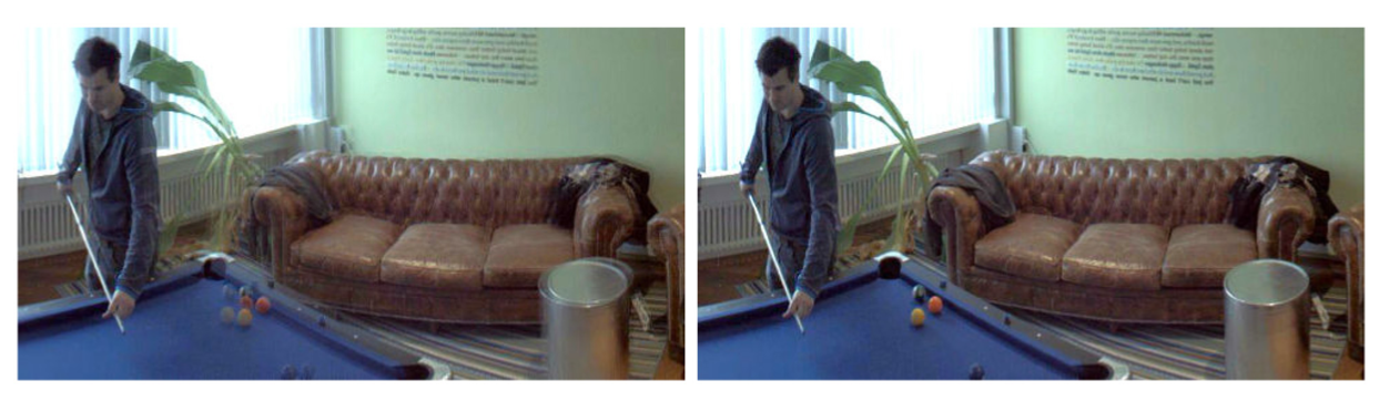
Virtual Head Motion. Our method produces accurate reconstructions, which enable a change of viewpoint. Figure 12 shows a close-up of different perspectives created from the same frame captured with our rig. For instance, the parallax between the foreground person and the metallic stool is clearly visible. By fixing points at infinity and animating, we can achieve an effect that corresponds to a sideways head motion. The accompanying video shows a real-time version of this effect displayed on an Oculus head mounted display.

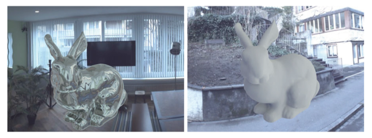
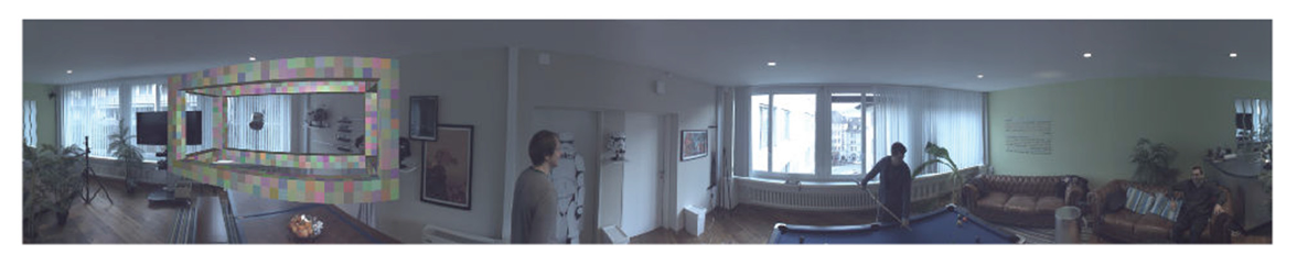
Compositing with CG. For mixing real-world and synthetic content in VR applications, it is straightforward to use the output panorama frames as dynamically changing environment maps for illuminating synthetic objects or refraction mapping (see Figure 17 for two examples). To insert computer generated content into the output video panoramas, we use the projection derived in Section 5.1, which renders objects appropriately distorted in agreement with our panoramic non-linear projection (see Figure 18).

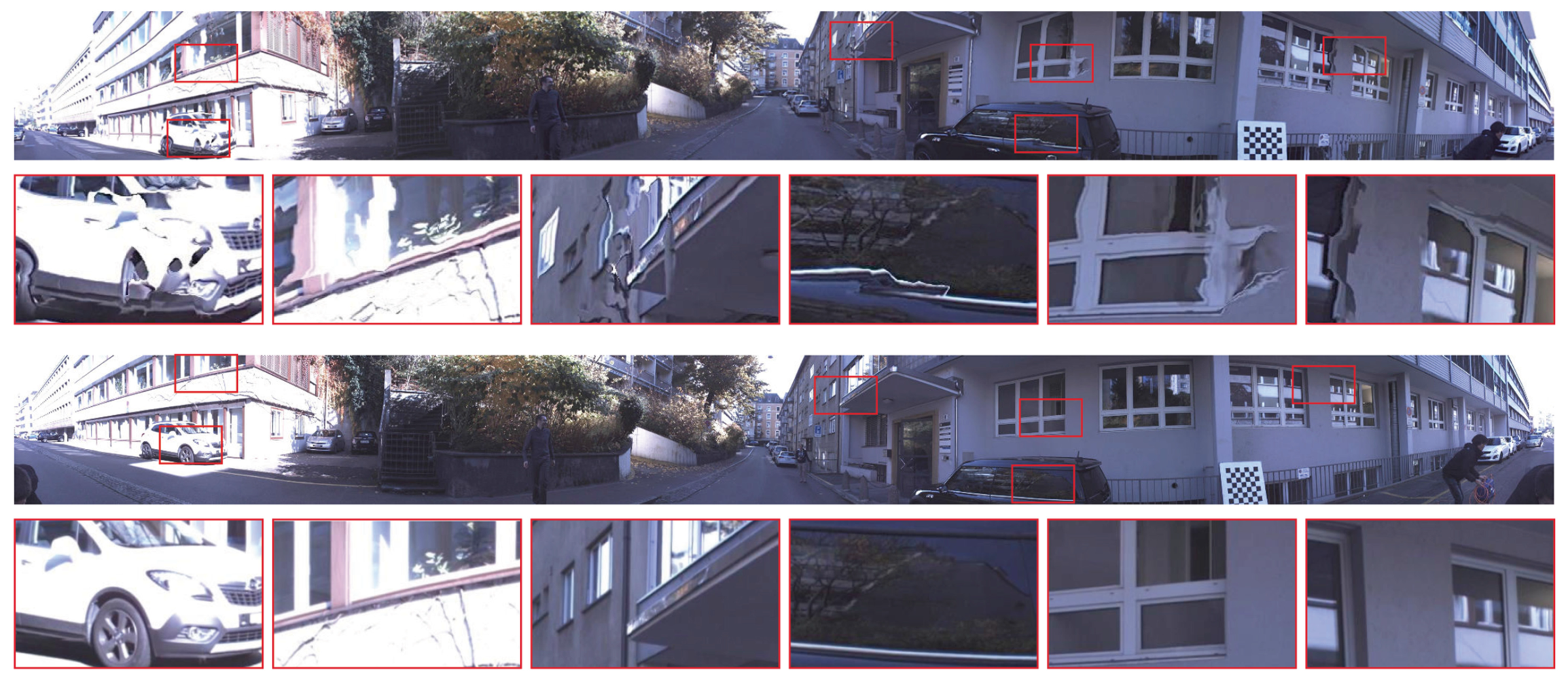
Comparison to a Depth-Based Pipeline. Our approach allows to create omnistereoscopic videos without explicit knowledge of scene geometry. However, if scene geometry was known, performing the view interpolation described in Section 4.2 would simply come down to rendering the scene with a common pinhole camera model as in Equation (3). Therefore, at a first glance, it may seem more desirable to follow a depth-based pipeline that estimates the 3D geometry of the scene and then reconstructs the desired lightfield by rendering novel views. We compare a depth-based result to ours in Figure 14.

In practice, a depth-based approach suffers from a number of drawbacks: The kind of camera rigs used for creating omnistereoscopic video are not suitable for the popular and commonly available multi-view stereo approaches such as [Fuhrmann et al. 2014], [Furukawa and Ponce 2009], [Galliani et al. 2015], and [Zhang et al. 2009], which all did not yield any useable results for our scenario. This may be due to the fact that such methods are rather tailored to scenarios where a large number of cameras observes a part of a scene from different locations as opposed to a relatively small number of cameras observing different parts of a scene from almost the same location.

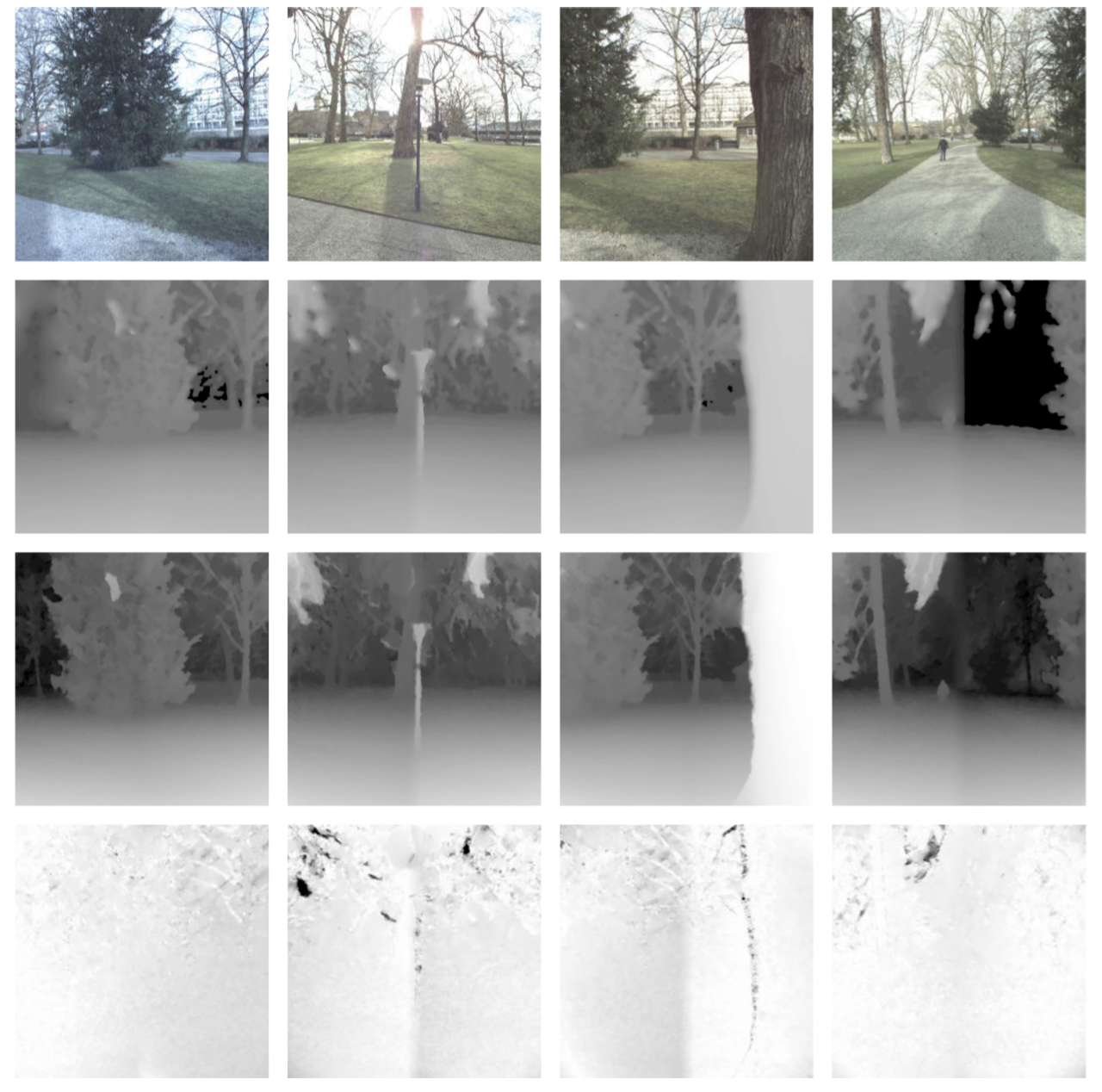
Thus, for a depth-based pipeline, we had to resort to a two-view stereo method. We used the OpenCV implementation of a commonly available state-of-the-art stereo algorithm [Hirschmuller 2007]. The depth map for a single camera is estimated in four steps: First, we select the reference camera and its left neighbor, perform a rectification, and compute stereo disparities. Second, we do the same for the reference camera and its right neighbor. In the third step, we convert the disparities to depth values using the cameras focal length and baselines, and blend them in the coordinate frame of the reference camera. In order to achieve a reasonable blending, we have to keep track of the overlap regions between camera pairs. In the fourth and last step, we fill in missing information in the depth map by performing inpainting. Figure 15 visualizes the depth map resulting from these computations for one of the input views.

Besides requiring multiple steps for obtaining a single depth-map, the depth-based approach is also much more dependent on accurate calibration information. In the extreme case where no calibration information is used, our flow-based approach is already able to produce photometrically accurate panoramas that only suffer from geometric distortion (as shown in Figure 11) while a depth-based approach is not applicable at all. The depth-based approach is sensitive to calibration errors since correspondences are only searched for along epipolar lines. Thus, stereo methods cannot deal with imperfections in the calibration and have less flexibility to resolve brittle situations that do not follow epipolar geometry. In contrast, pixel movement described by optical flow can often be sufficient and more stable in practice. The ability to deviate from epipolar constraints allows us to be more robust and remove ghosting artifacts, which leads to a visually more pleasing panoramic image (as shown in Figure 14). Figure 15 (bottom) illustrates how much the flow correspondences deviate from the epipolar constraints by visualizing our flow-based correspondences decomposed into magnitude along and across the epipolar line.

Relation to Google Jump. Google Jump [Anderson et al. 2016] and our work have been developed concurrently. Both can be seen as extensions of Megastereo [Richardt et al. 2013] to dynamic scenes. As such, they have to deal with an order of magnitude less input views. This makes the correspondence estimation, which is required for correct view interpolation, more difficult. Both works use flow correspondences instead of depth for view interpolation. While Google Jump uses block matching and the bilateral solver for filtering matches in a second step, we find correspondences by dense optical flow incorporating prealignment.

Besides this, we also derive the omnistereoscopic panorama generation from a view interpolation problem and quantify the deviation to geometric view interpolation that their and also our approach introduce in more detail (see Figure 7). This gives insight into deviations from geometric view interpolation with respect to the depth of a scene point for cameras with different fields of view, camera arrays with different numbers of cameras, and points with different elevations.

We also describe how to achieve a virtual head motion effect for sideways headmotion in VR and show results in our demo application using an Oculus Rift. Although we suggest using flow correspondences for view interpolation as in Google Jump, we also describe a depth-based approach for omnistereoscopic panorama generation and show comparisons between the depth-based and the flow-based approach. We also describe and show an example of how to correctly incorporate CG elements into the panorama (Figure 18).

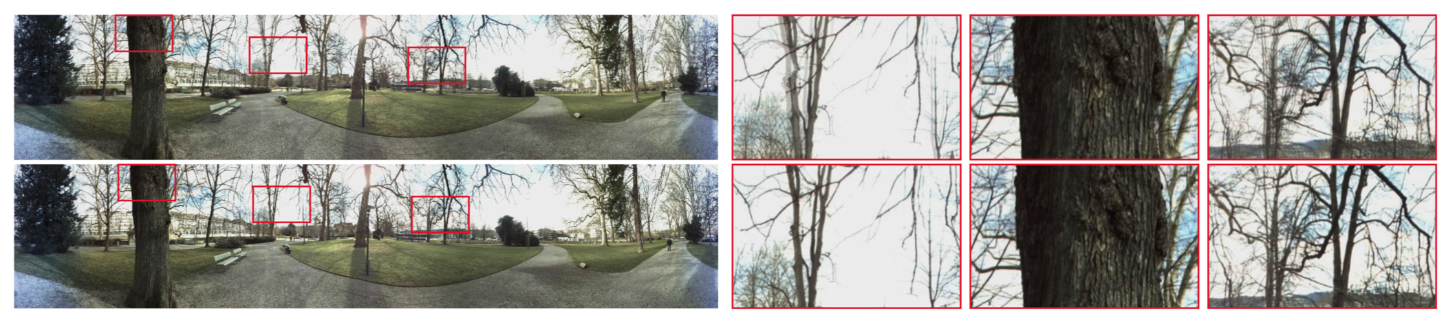
Comparison to Facebook Surround 360. Figure 16 compares our method to results obtained with Facebook’s recently released Surround 360 software (github.com/facebook/Surround360). We ran the full pipeline of Surround 360 including calibration steps such as the ring rectification and color adjustment. Furthermore, we supplied the intrinsic camera parameters that we also use in our algorithm. Judging by the source code, the ring rectification used in the Surround 360 algorithm jointly estimates a homography for every input camera in order to compensate for small deviations from an ideal camera setup, which would be obtained by evenly sampling α in Equation (3). However, the objective function used in the ring rectification step only penalizes deviations in the y-coordinate of corresponding points after projecting them on a spherical surface. Although the camera rig that we used (see Figure 9) is already quite close to such an ideal setup, compared to our approach the Surround 360 algorithm produces noticeable artifacts in many regions of the resulting panorama (see the close-ups in Figure 16).

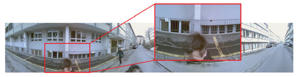
Limitations. Our approach has some limitations and potential directions for future work. Our study provides insight guidelines for scene acquisition (Section 5), for example, in terms of minimum scene depth. When the derived minimum depth is violated, ghosting effects appear (Figure 19).

The admissible range of virtual head motion depends on the radius of the camera array and the amount of camera overlap. To increase the overlap, a solution is to increase the number of cameras, which can become complicated in practice, or to use cameras with a wider field of view. Since a wider field of view corresponds to a loss in spatial resolution, a compromise has to be found in practice.

Creating a smooth head motion animation needs 10 to 20 panoramic image slices. Compared to the usual two slices required for common onmnistereo, this is up to an order of magnitude more data, which would make it difficult to use for video streaming. However, since there is a lot of redundancy in the data, it is optimally suited for efficient compression. Therefore, investigating compression approaches for such kind of data or also different representations of this data can be interesting directions for future research. There are also research opportunities for more principled future work, such as the extension of virtual head motion effects beyond sideways translation and handling the singularities at the poles.

7 CONCLUSION

A practically feasible approach for omnistereoscopic video capture and display of the real-world, including support for virtual head motion currently is one of the key hindrances to a more widespread adoption of real-world VR. In this article, we built on the concept of omnistereoscopic panoramas and described both, a practical way of capturing and generating the necessary image data from a sparse array of cameras, as well as an analysis of the system parameters and a practical guide to achieve plausible stereoscopic output. By sharing our new insights, we hope that this work facilitates the widespread adoption and creation of realworld VR, given that this is currently such a thriving and exciting area in both academia and industry.

8 ACKNOWLEDGMENTS

We are very grateful to Henning Zimmer for his tremendous help with the acquisition and his expertise on optical flow. We also thank Max Grosse for his invaluable help with the Oculus Rift. We also would like to thank Maurizio Nitti for creating the Robot scene, Alessia Marra for the experiments with the environment maps, and Jan Wezel for his help with building the camera rigs.

9 REFERENCE