❤: Regularized
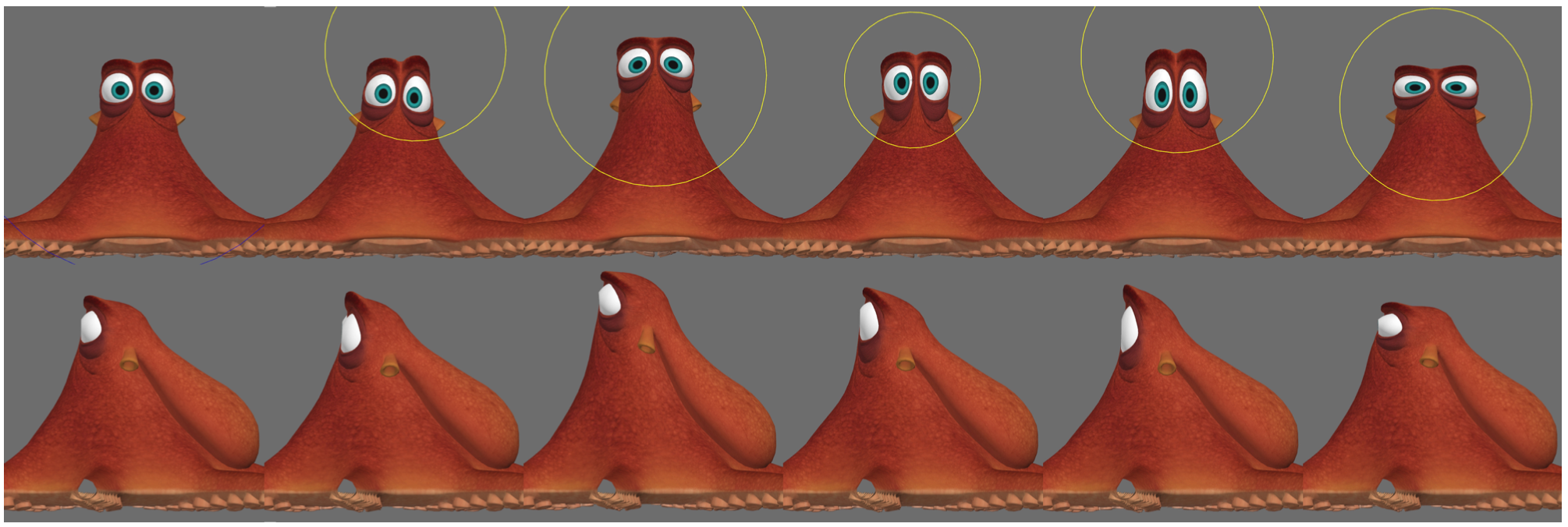 Fig.1. RegularizedKelvinlets: Examples of expressions generated by regularized Kelvinlets, a novel approach for sculpting that provides space deformations with real-time feedback and interactive volume control based on closed-form analytical solutions of linear elasticity. ©Disney/Pixar
# INTRODUCTION
Digital sculpting is a core component in modeling and animation packages, e.g., ZBrush, Scultpris, MudBox, Maya, or Modo. While purely geometric approaches are commonplace for shape editing, physically based deformers have long been sought to provide a more natural and effective sculpting tool for digital artists. However, existing physics-driven methods tend to have practical impediments for interactive design: they are inherently slow due to the need to numerically solve equations of the underlying discrete deformation model, and also involve tedious setup steps such as volumetric meshing, boundary condition specification, or preprocessing to accelerate the simulation.
In this paper, we introduce a novel sculpting tool that offers interactive and physically plausible deformations. Our approach is based on the regularization of the fundamental solutions to the equations of linear elasticity for specific brush-like forces (e.g., grab, twist, pinch) applied to a virtual infinite elastic space. Since the fundametal solutions of linear elasticity for singular loads are known as Kelvinlets [@phan1994microstructures], we refer to our new solutions as regularized Kelvinlets. This formulation leads to analytical closedform expressions, thus making our method free of any geometric discretization, computationally intensive solve, or large memory requirement. Instead, our brush-like deformations can be rapidly evaluated on the fly for sculpting sessions, with interactive control of the volume compression of the elastic material (Figure 1). To address the typical long-range falloffs of the fundamental solutions, we present a multi-scale extrapolation scheme that builds compound brushes with arbitrarily fast decay, thereby enabling highly localized edits. For more specialized control, we also propose a linear combination of brushes that imposes pointwise constraints on displacements and gradients through a single linear solve. In summary, regularized Kelvinlets offer volume-aware deformations that are efficient to evaluate, easy to parallelize, and complementary to existing modeling techniques.
# RELATED WORK
Sculpting methods for digital shapes have been investigated extensively in graphics, see survey in [@cani2006towards]. The most common sculpting tool is the family of grab/twist/scale/pinch brushes available in commercial modeling packages, e.g., [@Maya]. In these brushes, a single affine transformation is applied to every point in space and scaled by a predefined falloff. The simple setup and fast analytical evaluation make these tools suitable for highly detailed modeling, as well as animation and post-simulation edits. Motivated by these premises, our work augments existing brush deformations with interactive elastic response.
In order to provide volume-aware sculpts, [@angelidis2004sweepers] introduced the notion of sweeper brushes, which deform the space with no self-intersection by advecting points along user-authored displacement fields. This technique was later extended to swirling-sweepers [@angelidis2006swirling] that ensure constant-volume deformations by emulating the formation of vortex rings in incompressible fluids. Similarly, the work of [@von2006vector] proposed deformations with divergence-free displacements generated by user-designed scalar fields. Our approach shares similar properties with sweeper brushes, in particular, it guarantees foldover-free sculpts guided by displacement fields. However, we model a wider family of brush deformations that incorporates volumetric responses to elastic materials with compression. Also, instead of crafting functions that produce incompressible flows, we design smooth force distributions and rely on analytical solutions to the equations of elasticity to produce physically based deformations.
Solid modeling and carving were also explored using voxel discretizations [@galyean1991sculpting], sampled distance functions [@frisken2000adaptively], and adaptive resolution [@ferley2001resolution]. In [@dewaele2004interactive], physics-aware volume sculpting was addressed through voxel-based approximations of elastic and plastic deformations. However, these methods are restricted to grid-like data structures and tend to produce over-smoothed shapes. Other interactive techniques rely on user-controlled handles to drive volumetric deformations. This includes lattice deformers [@coquillart1990extended; @sederberg1986free], cage-based generalized barycentric coordinates [@joshi2007harmonic; @lipman2008green], linear blending skinning [@magnenat1988joint], wire curves [@singh1998wires], and sketch editing [@cordier2016sketch], to cite a few. In [@jacobson2011bounded], various handle types were supported by optimizing a unified linear blending scheme. In contrast to our work, these approaches require a careful placement of handles and a precomputation step that binds handles to the deforming objects. Moreover, the resulting deformations are purely geometric with limited volume control.
Aiming at physically plausible deformations, some methods combined handle-based systems with simulation techniques. For instance, [@jacobson2012fast] posed skinned skeletons by minimizing an elastic potential energy, while [@hahn2012rig] projected the equations of elasticity to the subspace spanned by animation rigs. In a similar way, the work of [@ben2009variational] deformed a cage mesh by optimizing the rigidity of the associated deformation. In [@kavan2012elasticity], an elasticity-inspired skinning was presented by constructing joint deformers. Physics-driven video editing was also considered by combining simulation with image aware constraints [Bazin et al. 2016]. It is also worth mentioning advances in elasticity solvers that speed up quasi-static simulations in 2D [@setaluri2015fast] and 3D [@mcadams2011efficient]. Model reduction can also make simulations orders of magnitude faster by precomputing deformation modes [@barbivc2005real] and multi-domain subspaces [@barbivc2011real]. Surface-only methods were also proposed to approximate elastic materials using, e.g., rigidity penalties [@sorkine2007rigid] and moving frames [@lipman2007volume]. Since these approaches rely on mesh discretizations and non-linear solvers, we consider them complementary to our mesh-free closed-form solutions.
Our work is closely related to the concept of regularized Stokeslets. Coined by [@hancock1953self], Stokeslets are singular fundamental solutions of Stokes flows (i.e., incompressible fluid flows with low Reynolds number [@chwang1975hydromechanics]) based on pointwise loads. To remove the singularity of these solutions, [@cortez2001method] introduced regularized Stokeslets as an alternative that replaces impulses by smoothed force distributions. Extensions to doublets and the method of images were later derived in [@ainley2008method; @cortez2005method], and employed to model the trajectories of self-propelled micro-organisms. Instead, we introduce the regularization of the fundamental solutions of linear elasticity, thus generalizing regularized Stokeslets to arbitrary elastic materials. In particular, our formulation reproduces regularized Stokeslets in the case of incompressible elasticity. In addition, we present a new approach to design regularized solutions with faster decays.
Finally, we point out that fundamental solutions are central to integral formulations of elasticity and discretizations such as the boundary element method (BEM) [@brebbia2012boundary]. In [@james1999artdefo], BEM was employed to deform surface meshes by approximating contact mechanics. However, this technique requires the precomputation and incremental updates of boundary conditions for displacements and surface tractions. This approach was later accelerated by compressing singular fundamental solutions of linear elasticity based on wavelets [@james2003multiresolution]. In contrast, we advocate the use of regularized fundamental solutions for digital sculpting, with no boundary specification or mesh discretization.
# BACKGROUND
Before presenting our new sculpting tools, we first review core concepts of linear elastostatics upon which our formulation is based. In the next sections, we focus our exposition on 3D linear elasticity and postpone the 2D case to Section 8, where the analogous 2D expressions are derived using our 3D results. For more details on linear elastostatics, we point the reader to [@slaughter2012linearized].
Elastostatics: In an infinite 3D continuum, the quasi-static equilibrium state of linear elasticity is determined by a displacement field $\boldsymbol{u} : R^3 → R^3$ that minimizes the elastic potential energy
$$
E(\boldsymbol{u})=\frac{\mu}{2}\|\nabla \boldsymbol{u}\|^{2}+\frac{\mu}{2(1-2 v)}\|\nabla \cdot \boldsymbol{u}\|^{2}-\langle\boldsymbol{b}, \boldsymbol{u}\rangle
$$
where ∥ · ∥ and ⟨·, ·⟩ are integrated over the infinite elastic volume. The first term in (1) controls the smoothness of the displacement field, the second term penalizes infinitesimal volume change, and the last term indicates the external body forces b to be counteracted. In this formulation, linear homogeneous and isotropic material parameters are given by the elastic shear modulus μ and the Poisson ratio ν. Note that, while the former is a simple scaling factor indicating the material stiffness, the latter dictates the material compressibility. By computing the critical point of (1), one can associate the optimal displacement field u with the solution of the well-known Navier-Cauchy equation (see, e.g., [@slaughter2012linearized]):
$$
\mu \Delta \boldsymbol{u}+\frac{\mu}{(1-2 v)} \nabla(\nabla \cdot \boldsymbol{u})+\boldsymbol{b}=0
$$
Kelvinlets: In the case of a concentrated body load due to a force vector $\boldsymbol{f}$ at a point $\boldsymbol{x}_0$, i.e., $\boldsymbol{b}(\boldsymbol{x}) = \boldsymbol{f} δ(\boldsymbol{x} −\boldsymbol{x}_0)$, the solution of (2) defines the (singular) fundamental solution of linear elasticity, also known as the Kelvin’s state [@kelvin1848note] or Kelvinlet [@phan1994microstructures], which can be written as
``` iheartla
`$\boldsymbol{u}$`(`$\boldsymbol{r}$`) = ((a-b)/rI_3 + b/r³ `$\boldsymbol{r}$` `$\boldsymbol{r}$`^T) `$\boldsymbol{f}$` where `$\boldsymbol{r}$` ∈ ℝ^3
where
r ∈ ℝ: the norm of $\boldsymbol{r}$
```
where $\boldsymbol{r} =\boldsymbol{x}−\boldsymbol{x}_0$ is the relative position vector from the load location $\boldsymbol{x}_0$ to an observation point $\boldsymbol{x}$, and $r = ∥\boldsymbol{r}∥$ is its norm. The coefficients in (3) are of the form $a=1/(4πμ)$ and $b=a/[4(1−ν)]$. Here, we refer to $K( \boldsymbol{r} )$ as the Green’s function for linear elasticity that defines a 3×3 matrix mapping the force vector $\boldsymbol{f}$ at $\boldsymbol{x}_0$ to the displacement vector $\boldsymbol{u}$ at a relative position $\boldsymbol{r}$ . Notice that the first term in $K( \boldsymbol{r} )$ resembles the Laplacian Green’s function scaled by a constant, while the second term controls volume compression by modifying the elastic response based on the alignment of the relative position vector $\boldsymbol{r}$ to the force vector $\boldsymbol{f}$ . Moreover, observe that no boundary conditions were needed for the definition of Kelvinlets, since these displacement fields are the minimizer of the elastic potential energy over the infinite space.
Stokeslets: An important special case of linear elastostatics occurs for incompressible materials, i.e., $ν = 1/2$. In this case, the divergence penalty term in (1) becomes a hard constraint $∇ · \boldsymbol{u}= 0$ that ensures incompressible displacements. The solution for this constrained minimization can be computed via the Stokes equation:
$$
\mu \Delta \boldsymbol{u}+\boldsymbol{b}-\nabla p=0 \quad \text { subject to } \quad \nabla \cdot \boldsymbol{u}=0
$$
where p is the pressure scalar field acting as a Lagrangian multiplier that enforces the divergence-free constraint. For a pointwise load with force vector $\boldsymbol{f}$ , the (singular) fundamental solution of (4) is known as the Stokeslet [@chwang1975hydromechanics; Hancock 1953], and matches the expression in (3) with ν =1/2 (i.e., b =a/2).
Deformation Gradient: From a displacement field $\boldsymbol{u}(\boldsymbol{x} −\boldsymbol{x}_0)$, an arbitrary point $\boldsymbol{x}$ embedded in a linear elastic material is deformed to $\boldsymbol{x} +\boldsymbol{u}(\boldsymbol{x} −\boldsymbol{x}_0)$. The associated deformation gradient is then defined by a 3×3 matrix of the form $\boldsymbol{G}(\boldsymbol{x}−\boldsymbol{x}_0)=\boldsymbol{I}+∇\boldsymbol{u}(\boldsymbol{x}−\boldsymbol{x}_0)$. By analyzing this matrix G(r), we can obtain different properties of the displacement field u(r) (see, e.g., [@slaughter2012linearized]). For instance, the skew-symmetric part of ∇u(r) indicates the infinitesimal rotation induced by u(r), while its symmetric part corresponds to the elastic strain and determines the infinitesimal stretching. The strain tensor can be also decomposed into a trace term that represents the uniform scaling of the volume of the elastic medium, and a traceless term that informs the undergoing pinching deformation. We will use these deformation gradient decompositions in Section 6 to construct twist, scale, and pinch elastic brushes.
# 3D REGULARIZED KELVINLETS
The concentrated body load at a single point $x_0$ introduces a singularity to the Kelvinlet solution, making its displacements and derivatives indefinite nearby $x_0$. For this reason, the singular Kelvinlet is numerically unsuitable for digital sculpting. To overcome this issue, we adopt the regularization scheme introduced in [@cortez2001method], and consider a smoothed body load $b(r)=fρ_ε(r)$ with force vector $f$ and normalized density function $ρ_ε(r)$ distributed around $x_0$ by a radial scale $ε > 0$. Similar to [@cortez2005method], we define the regularized distance $r_ε$ $ = √r^2+ε^2$ and set the normalized density function ${\rho}_ε ( \boldsymbol{r} )$ to be of the form (see inset)
``` iheartla
`${\rho}_ε$`(`$\boldsymbol{r}$`) = (15`$r_ε$`^4/(8π) + 1/`$r_ε$`^7 ) where `$\boldsymbol{r}$` ∈ ℝ^3
```
Fig.1. RegularizedKelvinlets: Examples of expressions generated by regularized Kelvinlets, a novel approach for sculpting that provides space deformations with real-time feedback and interactive volume control based on closed-form analytical solutions of linear elasticity. ©Disney/Pixar
# INTRODUCTION
Digital sculpting is a core component in modeling and animation packages, e.g., ZBrush, Scultpris, MudBox, Maya, or Modo. While purely geometric approaches are commonplace for shape editing, physically based deformers have long been sought to provide a more natural and effective sculpting tool for digital artists. However, existing physics-driven methods tend to have practical impediments for interactive design: they are inherently slow due to the need to numerically solve equations of the underlying discrete deformation model, and also involve tedious setup steps such as volumetric meshing, boundary condition specification, or preprocessing to accelerate the simulation.
In this paper, we introduce a novel sculpting tool that offers interactive and physically plausible deformations. Our approach is based on the regularization of the fundamental solutions to the equations of linear elasticity for specific brush-like forces (e.g., grab, twist, pinch) applied to a virtual infinite elastic space. Since the fundametal solutions of linear elasticity for singular loads are known as Kelvinlets [@phan1994microstructures], we refer to our new solutions as regularized Kelvinlets. This formulation leads to analytical closedform expressions, thus making our method free of any geometric discretization, computationally intensive solve, or large memory requirement. Instead, our brush-like deformations can be rapidly evaluated on the fly for sculpting sessions, with interactive control of the volume compression of the elastic material (Figure 1). To address the typical long-range falloffs of the fundamental solutions, we present a multi-scale extrapolation scheme that builds compound brushes with arbitrarily fast decay, thereby enabling highly localized edits. For more specialized control, we also propose a linear combination of brushes that imposes pointwise constraints on displacements and gradients through a single linear solve. In summary, regularized Kelvinlets offer volume-aware deformations that are efficient to evaluate, easy to parallelize, and complementary to existing modeling techniques.
# RELATED WORK
Sculpting methods for digital shapes have been investigated extensively in graphics, see survey in [@cani2006towards]. The most common sculpting tool is the family of grab/twist/scale/pinch brushes available in commercial modeling packages, e.g., [@Maya]. In these brushes, a single affine transformation is applied to every point in space and scaled by a predefined falloff. The simple setup and fast analytical evaluation make these tools suitable for highly detailed modeling, as well as animation and post-simulation edits. Motivated by these premises, our work augments existing brush deformations with interactive elastic response.
In order to provide volume-aware sculpts, [@angelidis2004sweepers] introduced the notion of sweeper brushes, which deform the space with no self-intersection by advecting points along user-authored displacement fields. This technique was later extended to swirling-sweepers [@angelidis2006swirling] that ensure constant-volume deformations by emulating the formation of vortex rings in incompressible fluids. Similarly, the work of [@von2006vector] proposed deformations with divergence-free displacements generated by user-designed scalar fields. Our approach shares similar properties with sweeper brushes, in particular, it guarantees foldover-free sculpts guided by displacement fields. However, we model a wider family of brush deformations that incorporates volumetric responses to elastic materials with compression. Also, instead of crafting functions that produce incompressible flows, we design smooth force distributions and rely on analytical solutions to the equations of elasticity to produce physically based deformations.
Solid modeling and carving were also explored using voxel discretizations [@galyean1991sculpting], sampled distance functions [@frisken2000adaptively], and adaptive resolution [@ferley2001resolution]. In [@dewaele2004interactive], physics-aware volume sculpting was addressed through voxel-based approximations of elastic and plastic deformations. However, these methods are restricted to grid-like data structures and tend to produce over-smoothed shapes. Other interactive techniques rely on user-controlled handles to drive volumetric deformations. This includes lattice deformers [@coquillart1990extended; @sederberg1986free], cage-based generalized barycentric coordinates [@joshi2007harmonic; @lipman2008green], linear blending skinning [@magnenat1988joint], wire curves [@singh1998wires], and sketch editing [@cordier2016sketch], to cite a few. In [@jacobson2011bounded], various handle types were supported by optimizing a unified linear blending scheme. In contrast to our work, these approaches require a careful placement of handles and a precomputation step that binds handles to the deforming objects. Moreover, the resulting deformations are purely geometric with limited volume control.
Aiming at physically plausible deformations, some methods combined handle-based systems with simulation techniques. For instance, [@jacobson2012fast] posed skinned skeletons by minimizing an elastic potential energy, while [@hahn2012rig] projected the equations of elasticity to the subspace spanned by animation rigs. In a similar way, the work of [@ben2009variational] deformed a cage mesh by optimizing the rigidity of the associated deformation. In [@kavan2012elasticity], an elasticity-inspired skinning was presented by constructing joint deformers. Physics-driven video editing was also considered by combining simulation with image aware constraints [Bazin et al. 2016]. It is also worth mentioning advances in elasticity solvers that speed up quasi-static simulations in 2D [@setaluri2015fast] and 3D [@mcadams2011efficient]. Model reduction can also make simulations orders of magnitude faster by precomputing deformation modes [@barbivc2005real] and multi-domain subspaces [@barbivc2011real]. Surface-only methods were also proposed to approximate elastic materials using, e.g., rigidity penalties [@sorkine2007rigid] and moving frames [@lipman2007volume]. Since these approaches rely on mesh discretizations and non-linear solvers, we consider them complementary to our mesh-free closed-form solutions.
Our work is closely related to the concept of regularized Stokeslets. Coined by [@hancock1953self], Stokeslets are singular fundamental solutions of Stokes flows (i.e., incompressible fluid flows with low Reynolds number [@chwang1975hydromechanics]) based on pointwise loads. To remove the singularity of these solutions, [@cortez2001method] introduced regularized Stokeslets as an alternative that replaces impulses by smoothed force distributions. Extensions to doublets and the method of images were later derived in [@ainley2008method; @cortez2005method], and employed to model the trajectories of self-propelled micro-organisms. Instead, we introduce the regularization of the fundamental solutions of linear elasticity, thus generalizing regularized Stokeslets to arbitrary elastic materials. In particular, our formulation reproduces regularized Stokeslets in the case of incompressible elasticity. In addition, we present a new approach to design regularized solutions with faster decays.
Finally, we point out that fundamental solutions are central to integral formulations of elasticity and discretizations such as the boundary element method (BEM) [@brebbia2012boundary]. In [@james1999artdefo], BEM was employed to deform surface meshes by approximating contact mechanics. However, this technique requires the precomputation and incremental updates of boundary conditions for displacements and surface tractions. This approach was later accelerated by compressing singular fundamental solutions of linear elasticity based on wavelets [@james2003multiresolution]. In contrast, we advocate the use of regularized fundamental solutions for digital sculpting, with no boundary specification or mesh discretization.
# BACKGROUND
Before presenting our new sculpting tools, we first review core concepts of linear elastostatics upon which our formulation is based. In the next sections, we focus our exposition on 3D linear elasticity and postpone the 2D case to Section 8, where the analogous 2D expressions are derived using our 3D results. For more details on linear elastostatics, we point the reader to [@slaughter2012linearized].
Elastostatics: In an infinite 3D continuum, the quasi-static equilibrium state of linear elasticity is determined by a displacement field $\boldsymbol{u} : R^3 → R^3$ that minimizes the elastic potential energy
$$
E(\boldsymbol{u})=\frac{\mu}{2}\|\nabla \boldsymbol{u}\|^{2}+\frac{\mu}{2(1-2 v)}\|\nabla \cdot \boldsymbol{u}\|^{2}-\langle\boldsymbol{b}, \boldsymbol{u}\rangle
$$
where ∥ · ∥ and ⟨·, ·⟩ are integrated over the infinite elastic volume. The first term in (1) controls the smoothness of the displacement field, the second term penalizes infinitesimal volume change, and the last term indicates the external body forces b to be counteracted. In this formulation, linear homogeneous and isotropic material parameters are given by the elastic shear modulus μ and the Poisson ratio ν. Note that, while the former is a simple scaling factor indicating the material stiffness, the latter dictates the material compressibility. By computing the critical point of (1), one can associate the optimal displacement field u with the solution of the well-known Navier-Cauchy equation (see, e.g., [@slaughter2012linearized]):
$$
\mu \Delta \boldsymbol{u}+\frac{\mu}{(1-2 v)} \nabla(\nabla \cdot \boldsymbol{u})+\boldsymbol{b}=0
$$
Kelvinlets: In the case of a concentrated body load due to a force vector $\boldsymbol{f}$ at a point $\boldsymbol{x}_0$, i.e., $\boldsymbol{b}(\boldsymbol{x}) = \boldsymbol{f} δ(\boldsymbol{x} −\boldsymbol{x}_0)$, the solution of (2) defines the (singular) fundamental solution of linear elasticity, also known as the Kelvin’s state [@kelvin1848note] or Kelvinlet [@phan1994microstructures], which can be written as
``` iheartla
`$\boldsymbol{u}$`(`$\boldsymbol{r}$`) = ((a-b)/rI_3 + b/r³ `$\boldsymbol{r}$` `$\boldsymbol{r}$`^T) `$\boldsymbol{f}$` where `$\boldsymbol{r}$` ∈ ℝ^3
where
r ∈ ℝ: the norm of $\boldsymbol{r}$
```
where $\boldsymbol{r} =\boldsymbol{x}−\boldsymbol{x}_0$ is the relative position vector from the load location $\boldsymbol{x}_0$ to an observation point $\boldsymbol{x}$, and $r = ∥\boldsymbol{r}∥$ is its norm. The coefficients in (3) are of the form $a=1/(4πμ)$ and $b=a/[4(1−ν)]$. Here, we refer to $K( \boldsymbol{r} )$ as the Green’s function for linear elasticity that defines a 3×3 matrix mapping the force vector $\boldsymbol{f}$ at $\boldsymbol{x}_0$ to the displacement vector $\boldsymbol{u}$ at a relative position $\boldsymbol{r}$ . Notice that the first term in $K( \boldsymbol{r} )$ resembles the Laplacian Green’s function scaled by a constant, while the second term controls volume compression by modifying the elastic response based on the alignment of the relative position vector $\boldsymbol{r}$ to the force vector $\boldsymbol{f}$ . Moreover, observe that no boundary conditions were needed for the definition of Kelvinlets, since these displacement fields are the minimizer of the elastic potential energy over the infinite space.
Stokeslets: An important special case of linear elastostatics occurs for incompressible materials, i.e., $ν = 1/2$. In this case, the divergence penalty term in (1) becomes a hard constraint $∇ · \boldsymbol{u}= 0$ that ensures incompressible displacements. The solution for this constrained minimization can be computed via the Stokes equation:
$$
\mu \Delta \boldsymbol{u}+\boldsymbol{b}-\nabla p=0 \quad \text { subject to } \quad \nabla \cdot \boldsymbol{u}=0
$$
where p is the pressure scalar field acting as a Lagrangian multiplier that enforces the divergence-free constraint. For a pointwise load with force vector $\boldsymbol{f}$ , the (singular) fundamental solution of (4) is known as the Stokeslet [@chwang1975hydromechanics; Hancock 1953], and matches the expression in (3) with ν =1/2 (i.e., b =a/2).
Deformation Gradient: From a displacement field $\boldsymbol{u}(\boldsymbol{x} −\boldsymbol{x}_0)$, an arbitrary point $\boldsymbol{x}$ embedded in a linear elastic material is deformed to $\boldsymbol{x} +\boldsymbol{u}(\boldsymbol{x} −\boldsymbol{x}_0)$. The associated deformation gradient is then defined by a 3×3 matrix of the form $\boldsymbol{G}(\boldsymbol{x}−\boldsymbol{x}_0)=\boldsymbol{I}+∇\boldsymbol{u}(\boldsymbol{x}−\boldsymbol{x}_0)$. By analyzing this matrix G(r), we can obtain different properties of the displacement field u(r) (see, e.g., [@slaughter2012linearized]). For instance, the skew-symmetric part of ∇u(r) indicates the infinitesimal rotation induced by u(r), while its symmetric part corresponds to the elastic strain and determines the infinitesimal stretching. The strain tensor can be also decomposed into a trace term that represents the uniform scaling of the volume of the elastic medium, and a traceless term that informs the undergoing pinching deformation. We will use these deformation gradient decompositions in Section 6 to construct twist, scale, and pinch elastic brushes.
# 3D REGULARIZED KELVINLETS
The concentrated body load at a single point $x_0$ introduces a singularity to the Kelvinlet solution, making its displacements and derivatives indefinite nearby $x_0$. For this reason, the singular Kelvinlet is numerically unsuitable for digital sculpting. To overcome this issue, we adopt the regularization scheme introduced in [@cortez2001method], and consider a smoothed body load $b(r)=fρ_ε(r)$ with force vector $f$ and normalized density function $ρ_ε(r)$ distributed around $x_0$ by a radial scale $ε > 0$. Similar to [@cortez2005method], we define the regularized distance $r_ε$ $ = √r^2+ε^2$ and set the normalized density function ${\rho}_ε ( \boldsymbol{r} )$ to be of the form (see inset)
``` iheartla
`${\rho}_ε$`(`$\boldsymbol{r}$`) = (15`$r_ε$`^4/(8π) + 1/`$r_ε$`^7 ) where `$\boldsymbol{r}$` ∈ ℝ^3
```
 As detailed in Appendix A, the solution to the elastostatics equation (2) associated with the load distribution (5) corresponds to
``` iheartla
`$\boldsymbol{u}_ε$`(`$\boldsymbol{r}$`) = ((a-b)/`$r_ε$`I_3 + b/`$r_ε$`³ `$\boldsymbol{r}$` `$\boldsymbol{r}$`^T + aε²/(2`$r_ε$`³) I_3 ) `$\boldsymbol{f}$` where `$\boldsymbol{r}$` ∈ ℝ^3
where
`$\boldsymbol{f}$` ∈ ℝ^3: force vector
```
This solution, which we name regularized Kelvinlet, forms the building block of our sculpting technique. Compared to (3), the regularized Kelvinlet includes an extra $\varepsilon^{2} / r_{\varepsilon}^{3}$ term, and reproduces the singular case as the radial scale ε approaches zero. Moreover, the undesirable $1/r$ singularity of Kelvinlets is now regularized at r = 0 using a $1/r_{\varepsilon}$ term, while keeping the O(1/r) asymptotic decay as r → ∞. Therefore, the resulting displacements are finite, differentiable, and localized around $x_0$. One can also verify that the deformation gradient at $x_0$ is trivial, i.e., $\nabla \boldsymbol{u}_ε (0)=0$, implying that the deformation at the point under the load is locally rigid. It is also worth mentioning that different density functions (and thereby regularized solutions) could be used, and our choice is based on the formulation of regularized Stokeslets [@cortez2005method]. In fact, one can easily verify that the regularized Kelvinlets simplify to the regularized Stokeslets in the incompressible limit (ν = 1/2).
Equipped with the regularized Kelvinlets, we can now construct a sculpting brush that assigns the load center $x_0$ to the brush tip and sets the brush radius to ε . This indicates that, by increasing the brush size, the load distribution becomes wider. Given a force vector f , we can then evaluate the displacement generated by the regularized Kelvinlet analytically for every point in $R^3$. As a result, we can move points along this displacement field, thus defining our physically based space deformation. It is also convenient to parameterize the force vector f in terms of the brush tip displacement u. To this end, we expand (6) with the linear constraint $\boldsymbol{u}_{\varepsilon}(0)=\overline{\boldsymbol{u}}$, leading to
As detailed in Appendix A, the solution to the elastostatics equation (2) associated with the load distribution (5) corresponds to
``` iheartla
`$\boldsymbol{u}_ε$`(`$\boldsymbol{r}$`) = ((a-b)/`$r_ε$`I_3 + b/`$r_ε$`³ `$\boldsymbol{r}$` `$\boldsymbol{r}$`^T + aε²/(2`$r_ε$`³) I_3 ) `$\boldsymbol{f}$` where `$\boldsymbol{r}$` ∈ ℝ^3
where
`$\boldsymbol{f}$` ∈ ℝ^3: force vector
```
This solution, which we name regularized Kelvinlet, forms the building block of our sculpting technique. Compared to (3), the regularized Kelvinlet includes an extra $\varepsilon^{2} / r_{\varepsilon}^{3}$ term, and reproduces the singular case as the radial scale ε approaches zero. Moreover, the undesirable $1/r$ singularity of Kelvinlets is now regularized at r = 0 using a $1/r_{\varepsilon}$ term, while keeping the O(1/r) asymptotic decay as r → ∞. Therefore, the resulting displacements are finite, differentiable, and localized around $x_0$. One can also verify that the deformation gradient at $x_0$ is trivial, i.e., $\nabla \boldsymbol{u}_ε (0)=0$, implying that the deformation at the point under the load is locally rigid. It is also worth mentioning that different density functions (and thereby regularized solutions) could be used, and our choice is based on the formulation of regularized Stokeslets [@cortez2005method]. In fact, one can easily verify that the regularized Kelvinlets simplify to the regularized Stokeslets in the incompressible limit (ν = 1/2).
Equipped with the regularized Kelvinlets, we can now construct a sculpting brush that assigns the load center $x_0$ to the brush tip and sets the brush radius to ε . This indicates that, by increasing the brush size, the load distribution becomes wider. Given a force vector f , we can then evaluate the displacement generated by the regularized Kelvinlet analytically for every point in $R^3$. As a result, we can move points along this displacement field, thus defining our physically based space deformation. It is also convenient to parameterize the force vector f in terms of the brush tip displacement u. To this end, we expand (6) with the linear constraint $\boldsymbol{u}_{\varepsilon}(0)=\overline{\boldsymbol{u}}$, leading to
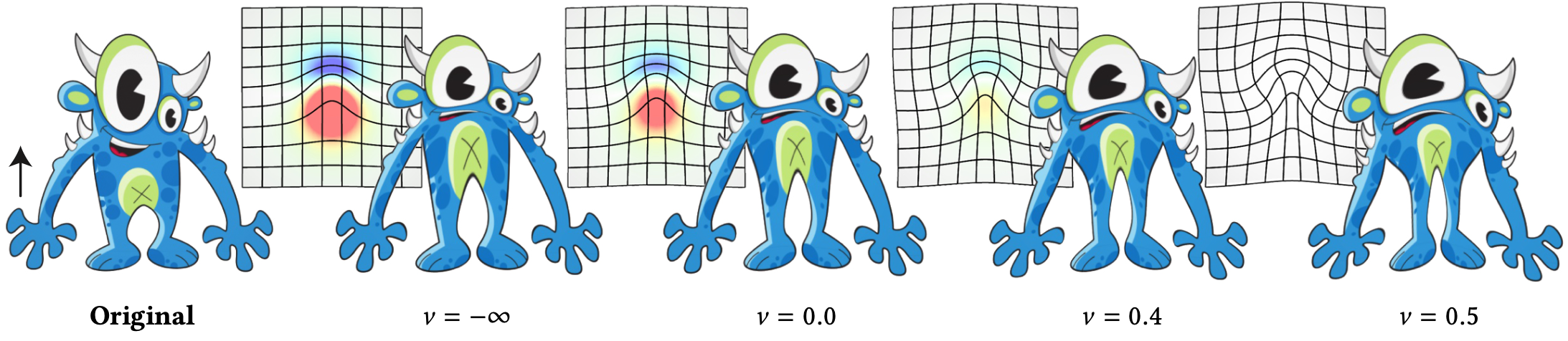 Fig. 2. Elastic Grab Brush: Regularized Kelvinlets offer interactive elastic response to grab displacements. This example shows the result of a bi-scale sculpting brush in 2D computed with a series of Poisson ratio values ν . Notice how larger values of ν lead to more bulging, e.g., along the body silhouette. The grid plots illustrate the local area loss and gain associated with different Poisson ratios. The pseudocolors encode a range from compression of 50% (blue) to dilation of 50% (red) relative to the rest area. Input image courtesy of Mirela Ben-Chen.
$$
\boldsymbol{u}_ε(\boldsymbol{r})=c ε \mathcal{K}_ε(\boldsymbol{r}) \overline{\boldsymbol{u}}
$$
where c =2/(3a − 2b). Note that this parameterization makes our brush independent of the shear modulus μ, so the only material parameter affecting the deformation is the Poisson ratio ν . Figure 2 shows regularized Kelvinlet deformations with varying Poisson ratio. In particular, observe the increasing bulging as the elastic material becomes incompressible. At last, we point out that, by setting the (unphysical but feasible) value ν = ±∞, the second term in (6) is annihilated and our displacement field simplifies to a typical grab brush with radial falloff available in commertical packages [Autodesk 2016], thus confirming that regularized Kelvinlets enrich existing grab brushes with elastic response.
# MULTI-SCALE EXTRAPOLATION
Sculpting brushes are commonly accompanied by falloff profiles that define the locality of the deformations. Generally, these functions are set independently of the brush operation and can even be adjusted by the user. In contrast, the spatial decay of regularized Kelvinlets is determined completely by the equations of linear elasticity. This fixed falloff may make our elastic deformations inadequate for fine sculpts in which a faster decay is demanded. To address this issue, we present next an extrapolation scheme that constructs physically based brushes with arbitrarily fast decays by linearly combining regularized Kelvinlets of different radial scales. Due to the superposition principle, these compound brushes form high-order regularized Kelvinlets that satisfy (2).
Asymptotic analysis: To better understand the far-field decay of a regularized Kelvinlet uε (r ), we analyzed the asymptotic expansion of the matrix Kε (r ) as r → ∞, whose first terms are
$$
C_{1}(\hat{\boldsymbol{r}})(1 / r)+ε^{2} C_{3}(\hat{\boldsymbol{r}})\left(1 / r^{3}\right)+ε^{4} C_{5}(\hat{\boldsymbol{r}})\left(1 / r^{5}\right)+O\left(1 / r^{7}\right)
\notag
$$
where the coefficients Ci (rˆ) indicate 3×3 matrices in terms of the normalized relative position rˆ = r /r , and material parameters μ and ν . (Formulas for Ci (rˆ) are provided in the supplemental material.) This expansion reveals an O(1/r) leading-order decay followed by odd powers of 1/r and even powers of ε. By properly combining n regularized Kelvinlet matrices Kεi (r) with different εi values, we can cancel the leading n − 1 terms and hasten the displacement falloff. This process is analogous to classical Richardson extrapolation for eliminating leading-order error terms in numerical differentiation [Brezinski and Zaglia 2013].
Bi-scale extrapolation: The simplest case of extrapolation is the difference of two regularized Kelvinlets of radii ε1 <ε2:
$$
\boldsymbol{u}_{ε_{1}, ε_{2}}(\boldsymbol{r})=\left[\mathcal{K}_{ε_{1}}(\boldsymbol{r})-\mathcal{K}_{ε_{2}}(\boldsymbol{r})\right] \boldsymbol{f}
$$
This solution corresponds to the physical response to two body loads applied at the same location, where the force pushing the smaller ε1-region is compensated by an equal but opposite pull over a spatially larger ε2-region. We can then consider the bi-scale extrapolation as an approximation of the first derivative of uε with respect to ε. From the asymptotic expansion, we observe that the first term cancels and the net result has a leading-order decay of O(1/r3), much faster than a single regularized Kelvinlet. We can also reproduce the tip displacement u by parameterizing the force vector f via the linear constraint uε1,ε2 (0)=u, yielding
$$
\boldsymbol{u}_{ε_{1}, ε_{2}}(\boldsymbol{r})=c\left(1 / ε_{1}-1 / ε_{2}\right)^{-1}\left[\mathcal{K}_{ε_{1}}(\boldsymbol{r})-\mathcal{K}_{ε_{2}}(\boldsymbol{r})\right] \overline{\boldsymbol{u}}
$$
Tri-scale extrapolation: Even greater locality of order O(1/r5) can
be generated by employing a tri-scale extrapolation:
$$
\boldsymbol{u}_{ε_{1}, ε_{2}, ε_{3}}(\boldsymbol{r})=\left[w_{1} \mathcal{K}_{ε_{1}}(\boldsymbol{r})+w_{2} \mathcal{K}_{ε_{2}}(\boldsymbol{r})+w_{3} \mathcal{K}_{ε_{3}}(\boldsymbol{r})\right] \boldsymbol{f}
$$
with distinct radial scales ε1 < ε2 < ε3 and weights w1,w2,w3. By analyzing its asymptotic expansion, we obtain
$$
\left(\sum_{i} w_{i}\right) C_{1}(\hat{\boldsymbol{r}})(1 / r)+\left(\sum_{i} w_{i} ε_{i}^{2}\right) C_{3}(\hat{\boldsymbol{r}})\left(1 / r^{3}\right)+O\left(1 / r^{5}\right)
\notag
$$
We can then cancel the two leading terms by setting the weights to
$$
w_{1}=1, w_{2}=-\left(ε_{3}^{2}-ε_{1}^{2}\right) /\left(ε_{3}^{2}-ε_{2}^{2}\right), w_{3}=\left(ε_{2}^{2}-ε_{1}^{2}\right) /\left(ε_{3}^{2}-ε_{2}^{2}\right)
\notag
$$
This solution provides an approximation of the second derivative of
uε with respect to ε. As before, we can parameterize the tri-scale
deformation in terms of tip displacement u, which takes the form
$$
\boldsymbol{u}_{ε_{1}, ε_{2}, ε_{3}}( \boldsymbol{r} )=c\left(\sum_{i} w_{i} / ε_{i}\right)^{-1}\left[\sum_{i} w_{i} \mathcal{K}_{ε_{i}}(\boldsymbol{r})\right] \overline{\boldsymbol{u}}
$$
Although a user may adjust each radial scale individually, setting ε2 and ε3 to small increments of ε1 leads to a better approximation of the derivatives of uε with respect to ε, thus creating a faster falloff in the proximity of the brush center and a high-order long-range decay. Therefore, we use εi +1 = 1.1εi as the default in our implementation, where ε1 corresponds to the brush radius. Figure 3 illustrates the different far-field decays generated by single, bi-scale, and tri-scale regularized Kelvinlets, all computed with the same tip displacement u. Figure 4 shows a closeup comparing the displacement field generated by a single-scale brush before and after reducing its radius ε by 50%, versus the result of increasing the falloff order to a tri-scale brush. Observe the significantly different decays of these displacement fields, despite of their similarity near the brush center. Finally, we point out that the multi-scale extrapolation can be continued indefinitely to produce brushes of arbitrarily high order decay and increasing locality.
Fig. 2. Elastic Grab Brush: Regularized Kelvinlets offer interactive elastic response to grab displacements. This example shows the result of a bi-scale sculpting brush in 2D computed with a series of Poisson ratio values ν . Notice how larger values of ν lead to more bulging, e.g., along the body silhouette. The grid plots illustrate the local area loss and gain associated with different Poisson ratios. The pseudocolors encode a range from compression of 50% (blue) to dilation of 50% (red) relative to the rest area. Input image courtesy of Mirela Ben-Chen.
$$
\boldsymbol{u}_ε(\boldsymbol{r})=c ε \mathcal{K}_ε(\boldsymbol{r}) \overline{\boldsymbol{u}}
$$
where c =2/(3a − 2b). Note that this parameterization makes our brush independent of the shear modulus μ, so the only material parameter affecting the deformation is the Poisson ratio ν . Figure 2 shows regularized Kelvinlet deformations with varying Poisson ratio. In particular, observe the increasing bulging as the elastic material becomes incompressible. At last, we point out that, by setting the (unphysical but feasible) value ν = ±∞, the second term in (6) is annihilated and our displacement field simplifies to a typical grab brush with radial falloff available in commertical packages [Autodesk 2016], thus confirming that regularized Kelvinlets enrich existing grab brushes with elastic response.
# MULTI-SCALE EXTRAPOLATION
Sculpting brushes are commonly accompanied by falloff profiles that define the locality of the deformations. Generally, these functions are set independently of the brush operation and can even be adjusted by the user. In contrast, the spatial decay of regularized Kelvinlets is determined completely by the equations of linear elasticity. This fixed falloff may make our elastic deformations inadequate for fine sculpts in which a faster decay is demanded. To address this issue, we present next an extrapolation scheme that constructs physically based brushes with arbitrarily fast decays by linearly combining regularized Kelvinlets of different radial scales. Due to the superposition principle, these compound brushes form high-order regularized Kelvinlets that satisfy (2).
Asymptotic analysis: To better understand the far-field decay of a regularized Kelvinlet uε (r ), we analyzed the asymptotic expansion of the matrix Kε (r ) as r → ∞, whose first terms are
$$
C_{1}(\hat{\boldsymbol{r}})(1 / r)+ε^{2} C_{3}(\hat{\boldsymbol{r}})\left(1 / r^{3}\right)+ε^{4} C_{5}(\hat{\boldsymbol{r}})\left(1 / r^{5}\right)+O\left(1 / r^{7}\right)
\notag
$$
where the coefficients Ci (rˆ) indicate 3×3 matrices in terms of the normalized relative position rˆ = r /r , and material parameters μ and ν . (Formulas for Ci (rˆ) are provided in the supplemental material.) This expansion reveals an O(1/r) leading-order decay followed by odd powers of 1/r and even powers of ε. By properly combining n regularized Kelvinlet matrices Kεi (r) with different εi values, we can cancel the leading n − 1 terms and hasten the displacement falloff. This process is analogous to classical Richardson extrapolation for eliminating leading-order error terms in numerical differentiation [Brezinski and Zaglia 2013].
Bi-scale extrapolation: The simplest case of extrapolation is the difference of two regularized Kelvinlets of radii ε1 <ε2:
$$
\boldsymbol{u}_{ε_{1}, ε_{2}}(\boldsymbol{r})=\left[\mathcal{K}_{ε_{1}}(\boldsymbol{r})-\mathcal{K}_{ε_{2}}(\boldsymbol{r})\right] \boldsymbol{f}
$$
This solution corresponds to the physical response to two body loads applied at the same location, where the force pushing the smaller ε1-region is compensated by an equal but opposite pull over a spatially larger ε2-region. We can then consider the bi-scale extrapolation as an approximation of the first derivative of uε with respect to ε. From the asymptotic expansion, we observe that the first term cancels and the net result has a leading-order decay of O(1/r3), much faster than a single regularized Kelvinlet. We can also reproduce the tip displacement u by parameterizing the force vector f via the linear constraint uε1,ε2 (0)=u, yielding
$$
\boldsymbol{u}_{ε_{1}, ε_{2}}(\boldsymbol{r})=c\left(1 / ε_{1}-1 / ε_{2}\right)^{-1}\left[\mathcal{K}_{ε_{1}}(\boldsymbol{r})-\mathcal{K}_{ε_{2}}(\boldsymbol{r})\right] \overline{\boldsymbol{u}}
$$
Tri-scale extrapolation: Even greater locality of order O(1/r5) can
be generated by employing a tri-scale extrapolation:
$$
\boldsymbol{u}_{ε_{1}, ε_{2}, ε_{3}}(\boldsymbol{r})=\left[w_{1} \mathcal{K}_{ε_{1}}(\boldsymbol{r})+w_{2} \mathcal{K}_{ε_{2}}(\boldsymbol{r})+w_{3} \mathcal{K}_{ε_{3}}(\boldsymbol{r})\right] \boldsymbol{f}
$$
with distinct radial scales ε1 < ε2 < ε3 and weights w1,w2,w3. By analyzing its asymptotic expansion, we obtain
$$
\left(\sum_{i} w_{i}\right) C_{1}(\hat{\boldsymbol{r}})(1 / r)+\left(\sum_{i} w_{i} ε_{i}^{2}\right) C_{3}(\hat{\boldsymbol{r}})\left(1 / r^{3}\right)+O\left(1 / r^{5}\right)
\notag
$$
We can then cancel the two leading terms by setting the weights to
$$
w_{1}=1, w_{2}=-\left(ε_{3}^{2}-ε_{1}^{2}\right) /\left(ε_{3}^{2}-ε_{2}^{2}\right), w_{3}=\left(ε_{2}^{2}-ε_{1}^{2}\right) /\left(ε_{3}^{2}-ε_{2}^{2}\right)
\notag
$$
This solution provides an approximation of the second derivative of
uε with respect to ε. As before, we can parameterize the tri-scale
deformation in terms of tip displacement u, which takes the form
$$
\boldsymbol{u}_{ε_{1}, ε_{2}, ε_{3}}( \boldsymbol{r} )=c\left(\sum_{i} w_{i} / ε_{i}\right)^{-1}\left[\sum_{i} w_{i} \mathcal{K}_{ε_{i}}(\boldsymbol{r})\right] \overline{\boldsymbol{u}}
$$
Although a user may adjust each radial scale individually, setting ε2 and ε3 to small increments of ε1 leads to a better approximation of the derivatives of uε with respect to ε, thus creating a faster falloff in the proximity of the brush center and a high-order long-range decay. Therefore, we use εi +1 = 1.1εi as the default in our implementation, where ε1 corresponds to the brush radius. Figure 3 illustrates the different far-field decays generated by single, bi-scale, and tri-scale regularized Kelvinlets, all computed with the same tip displacement u. Figure 4 shows a closeup comparing the displacement field generated by a single-scale brush before and after reducing its radius ε by 50%, versus the result of increasing the falloff order to a tri-scale brush. Observe the significantly different decays of these displacement fields, despite of their similarity near the brush center. Finally, we point out that the multi-scale extrapolation can be continued indefinitely to produce brushes of arbitrarily high order decay and increasing locality.
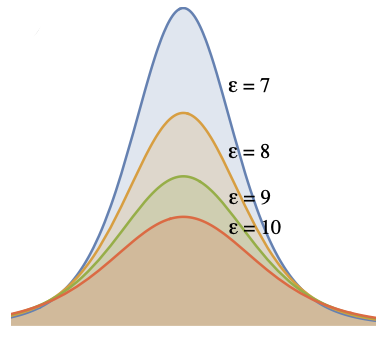
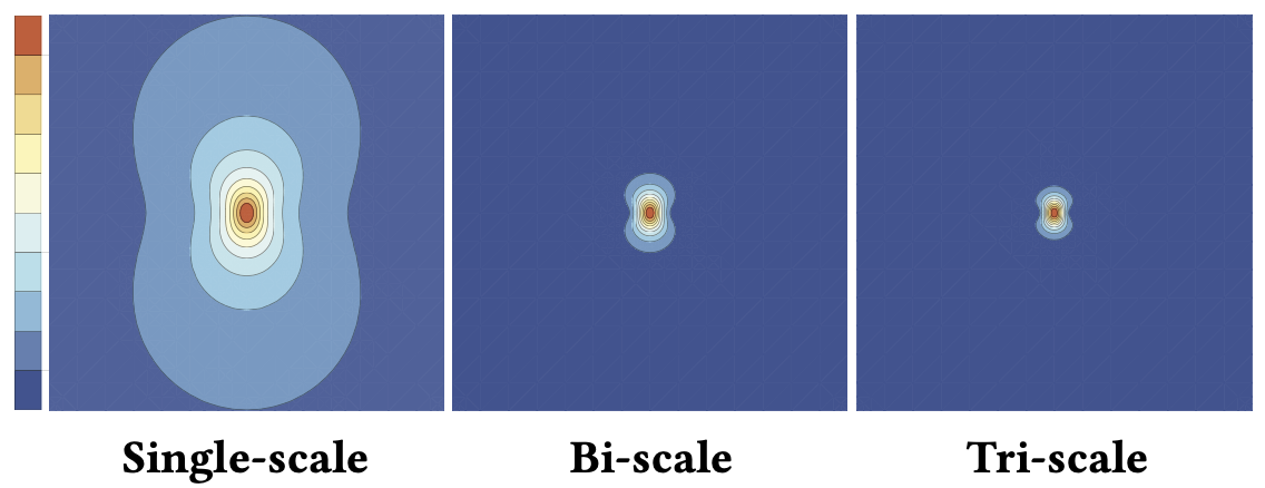 Fig. 3. Multi-scale extrapolation for fast decay: These plots display the contours of the norm of displacement fields generated by different multi-scale regularized Kelvinlets in 3D with ν =1/2. These brushes were parameterized by a unit displacement at the origin, thus leading to norm values in the inverval [0, 1]. Observe the long-range falloff of the single-scale brush, in contrast to the faster decays obtained by bi-scale and tri-scale brushes.
# EXTENSION TO AFFINE LOADS
So far we showed how to use regularized Kelvinlets to construct grablike deformations guided by the brush tip displacement. However, other sculpting operations assign an affine transformation, instead of a translation, to the brush. A typical example is the twist brush which defines a rotation centered at $x_0$. Similarly, scale and pinch brushes are generated based on affine transformations. In order to augment these brushes with elastic response, we propose to extend the formulation of regularized Kelvinlets by replacing the vector-based load distribution with a matrix-based distribution.
Fig. 3. Multi-scale extrapolation for fast decay: These plots display the contours of the norm of displacement fields generated by different multi-scale regularized Kelvinlets in 3D with ν =1/2. These brushes were parameterized by a unit displacement at the origin, thus leading to norm values in the inverval [0, 1]. Observe the long-range falloff of the single-scale brush, in contrast to the faster decays obtained by bi-scale and tri-scale brushes.
# EXTENSION TO AFFINE LOADS
So far we showed how to use regularized Kelvinlets to construct grablike deformations guided by the brush tip displacement. However, other sculpting operations assign an affine transformation, instead of a translation, to the brush. A typical example is the twist brush which defines a rotation centered at $x_0$. Similarly, scale and pinch brushes are generated based on affine transformations. In order to augment these brushes with elastic response, we propose to extend the formulation of regularized Kelvinlets by replacing the vector-based load distribution with a matrix-based distribution.
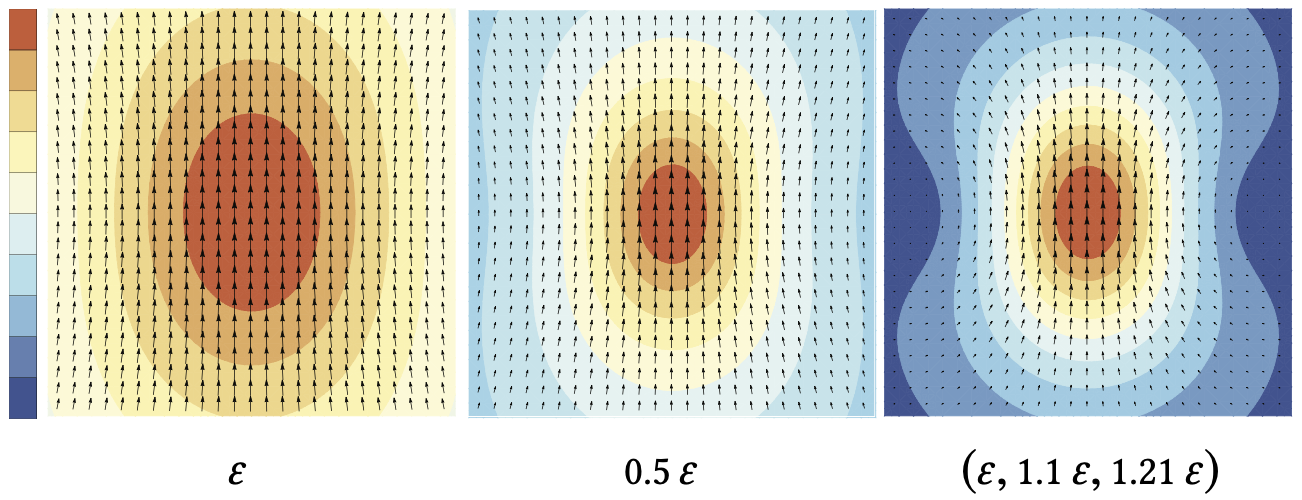 Fig. 4. Smaller radius vs. multi-scale extrapolation: A closeup of Figure 3 for a single-scale brush is shown overlaid by its displacement vectors (left). Reducing the brush radius ε makes the displacements more concentrated, but still with a long-range falloff (middle). In contrast, a tri-scale brush leads to localized displacements with a faster decay (right).
Our approach leverages the linearity of the elastostatics equation with respect to differentiation. More specifically, given a regularized Kelvinlet uε and its associated force vector f , we compute the directional derivative $\boldsymbol{g} \cdot \nabla$ of (2) along the vector $\boldsymbol{g}$, yielding
$$
\begin{aligned}
0 &=\boldsymbol{g} \cdot \nabla\left[\mu \Delta \boldsymbol{u}_ε+\frac{\mu}{(1-2 v)} \nabla\left(\nabla \cdot \boldsymbol{u}_ε\right)+\boldsymbol{b}\right] \\
&=\mu \Delta\left(\boldsymbol{g} \cdot \nabla \boldsymbol{u}_ε\right)+\frac{\mu}{(1-2 v)} \nabla\left[\nabla \cdot\left(\boldsymbol{g} \cdot \nabla \boldsymbol{u}_ε\right)\right]+\boldsymbol{g} \cdot \nabla \boldsymbol{b} \\
&=\mu \Delta \widetilde{\boldsymbol{u}}_ε+\frac{\mu}{(1-2 v)} \nabla\left[\nabla \cdot \widetilde{\boldsymbol{u}}_ε\right]+\widetilde{\boldsymbol{b}} .
\end{aligned}
\notag
$$
This implies that we can define a new body load $\widetilde{\boldsymbol{b}}(\boldsymbol{r})=\boldsymbol{g} \cdot \nabla \boldsymbol{b}(\boldsymbol{r})$ ,and its associated elastic response corresponds to the displacement field
$\tilde{\boldsymbol{u}}_ε(\boldsymbol{r})=g \cdot \nabla u_ε(\boldsymbol{r})$
We now consider the nine possible deformations $\tilde{\boldsymbol{u}}_ε^{i j}$ generated by setting $\boldsymbol{f} =\boldsymbol{e}_{i}$ and $\boldsymbol{g}=\boldsymbol{e}_{j}$ for every pair (i, j), where the vectors $\left\{\boldsymbol{e}_{1}, \boldsymbol{e}_{2}, \boldsymbol{e}_{3}\right\}$ form an orthonormal bases spanning $\mathbb{R}^{3}$. Due to super-position, we can linearly combine $\tilde{\boldsymbol{u}}_ε^{i j}$ with scalar coefficients $F_{i j}$, and obtain a matrix-driven solution of (2) of the form
$$
\widetilde{\boldsymbol{u}}_ε(\boldsymbol{r})=\sum_{i j} F_{i j} \boldsymbol{e}_{j} \cdot \nabla\left(\mathcal{K}_ε(\boldsymbol{r}) \boldsymbol{e}_{\boldsymbol{i}}\right)=\nabla \mathcal{K}_ε(\boldsymbol{r}): \boldsymbol{F}
$$
where $\boldsymbol{F} =\left[F_{i j}\right]$ is a 3×3 force matrix, and the symbol : indicates the double contraction of F to the third-order tensor $\nabla \mathcal{K}_ε(\boldsymbol{r})$, thus returning a vector. Similarly, we can write the body load that generates the deformation $\tilde{\boldsymbol{u}}_ε$ as
$$
\widetilde{\boldsymbol{b}}(\boldsymbol{r})=\sum_{i j} F_{i j} \boldsymbol{e}_{i} \boldsymbol{e}_{j}^{t} \nabla \rho_ε(\boldsymbol{r})= \boldsymbol{F} \nabla \rho_ε(\boldsymbol{r})
$$
By computing the spatial derivatives of $\boldsymbol{u}_ε$, we obtain the displacement field $\tilde{\boldsymbol{u}}_ε (\boldsymbol{r})$ in terms of the force matrix F :
``` iheartla
tr from linearalgebra
`$\tilde{\boldsymbol{u}}_ε$`(`$\boldsymbol{r}$`) = -a(1/`$r_ε$`³ + 3ε²/(2`$r_ε$`⁵) ) `$\boldsymbol{F}$``$\boldsymbol{r}$` + b(1/`$r_ε$`³(`$\boldsymbol{F}$`+`$\boldsymbol{F}$`^T+tr(`$\boldsymbol{F}$`)I_3) - 3/`$r_ε$`⁵(`$\boldsymbol{r}$`^T`$\boldsymbol{F}$``$\boldsymbol{r}$`)I_3)`$\boldsymbol{r}$` where `$\boldsymbol{r}$` ∈ ℝ^3
```
Note that the first term in (14) corresponds to an affine transformation $\boldsymbol{F} \boldsymbol{r}$ with a radial falloff similar to existing affine brushes, while the second term includes a symmetric affine transformation and controls volume compression through the Poisson ratio ν that b depends on. Therefore, we name this matrix-based extension of the fundamental solution of linear elasticity as a locally affine regularized Kelvinlet. For conciseness, we denote this displacement field by $\widetilde{u}_ε(\boldsymbol{r}) \equiv \mathcal{A}_ε(\boldsymbol{r}) \overrightarrow{\boldsymbol{F}}$, where $\overrightarrow{\boldsymbol{F}} \in \mathbb{R}^{9}$ is a vectorized form of F and $\mathcal{A}(\boldsymbol{r})$ is the 3×9 matrix that maps $\overrightarrow{\boldsymbol{F}}$ to a displacement at $\boldsymbol{r}$.
In contrast to (6), the deformation generated by (14) has zero displacement at the brush center, i.e., $\widetilde{\boldsymbol{u}}_ε(0)=0$, but a non-trivial gradient in terms of $\boldsymbol{F}$ (the closed-form expression is provided in the supplemental material). As the radial scale ε approaches zero, our matrix-based solutions reproduce the definition of Kelvinlet doublets [@phan1994microstructures]. These expressions also coincide with the regularized Stokeslet doublets [@ainley2008method] in the incompressible limit (ν = 1/2). Following the matrix decomposition in Section 3, we can further construct specialized versions of the locally affine regularized Kelvinlets by setting F to different types of matrices, as illustrated in Figure 5.
Fig. 4. Smaller radius vs. multi-scale extrapolation: A closeup of Figure 3 for a single-scale brush is shown overlaid by its displacement vectors (left). Reducing the brush radius ε makes the displacements more concentrated, but still with a long-range falloff (middle). In contrast, a tri-scale brush leads to localized displacements with a faster decay (right).
Our approach leverages the linearity of the elastostatics equation with respect to differentiation. More specifically, given a regularized Kelvinlet uε and its associated force vector f , we compute the directional derivative $\boldsymbol{g} \cdot \nabla$ of (2) along the vector $\boldsymbol{g}$, yielding
$$
\begin{aligned}
0 &=\boldsymbol{g} \cdot \nabla\left[\mu \Delta \boldsymbol{u}_ε+\frac{\mu}{(1-2 v)} \nabla\left(\nabla \cdot \boldsymbol{u}_ε\right)+\boldsymbol{b}\right] \\
&=\mu \Delta\left(\boldsymbol{g} \cdot \nabla \boldsymbol{u}_ε\right)+\frac{\mu}{(1-2 v)} \nabla\left[\nabla \cdot\left(\boldsymbol{g} \cdot \nabla \boldsymbol{u}_ε\right)\right]+\boldsymbol{g} \cdot \nabla \boldsymbol{b} \\
&=\mu \Delta \widetilde{\boldsymbol{u}}_ε+\frac{\mu}{(1-2 v)} \nabla\left[\nabla \cdot \widetilde{\boldsymbol{u}}_ε\right]+\widetilde{\boldsymbol{b}} .
\end{aligned}
\notag
$$
This implies that we can define a new body load $\widetilde{\boldsymbol{b}}(\boldsymbol{r})=\boldsymbol{g} \cdot \nabla \boldsymbol{b}(\boldsymbol{r})$ ,and its associated elastic response corresponds to the displacement field
$\tilde{\boldsymbol{u}}_ε(\boldsymbol{r})=g \cdot \nabla u_ε(\boldsymbol{r})$
We now consider the nine possible deformations $\tilde{\boldsymbol{u}}_ε^{i j}$ generated by setting $\boldsymbol{f} =\boldsymbol{e}_{i}$ and $\boldsymbol{g}=\boldsymbol{e}_{j}$ for every pair (i, j), where the vectors $\left\{\boldsymbol{e}_{1}, \boldsymbol{e}_{2}, \boldsymbol{e}_{3}\right\}$ form an orthonormal bases spanning $\mathbb{R}^{3}$. Due to super-position, we can linearly combine $\tilde{\boldsymbol{u}}_ε^{i j}$ with scalar coefficients $F_{i j}$, and obtain a matrix-driven solution of (2) of the form
$$
\widetilde{\boldsymbol{u}}_ε(\boldsymbol{r})=\sum_{i j} F_{i j} \boldsymbol{e}_{j} \cdot \nabla\left(\mathcal{K}_ε(\boldsymbol{r}) \boldsymbol{e}_{\boldsymbol{i}}\right)=\nabla \mathcal{K}_ε(\boldsymbol{r}): \boldsymbol{F}
$$
where $\boldsymbol{F} =\left[F_{i j}\right]$ is a 3×3 force matrix, and the symbol : indicates the double contraction of F to the third-order tensor $\nabla \mathcal{K}_ε(\boldsymbol{r})$, thus returning a vector. Similarly, we can write the body load that generates the deformation $\tilde{\boldsymbol{u}}_ε$ as
$$
\widetilde{\boldsymbol{b}}(\boldsymbol{r})=\sum_{i j} F_{i j} \boldsymbol{e}_{i} \boldsymbol{e}_{j}^{t} \nabla \rho_ε(\boldsymbol{r})= \boldsymbol{F} \nabla \rho_ε(\boldsymbol{r})
$$
By computing the spatial derivatives of $\boldsymbol{u}_ε$, we obtain the displacement field $\tilde{\boldsymbol{u}}_ε (\boldsymbol{r})$ in terms of the force matrix F :
``` iheartla
tr from linearalgebra
`$\tilde{\boldsymbol{u}}_ε$`(`$\boldsymbol{r}$`) = -a(1/`$r_ε$`³ + 3ε²/(2`$r_ε$`⁵) ) `$\boldsymbol{F}$``$\boldsymbol{r}$` + b(1/`$r_ε$`³(`$\boldsymbol{F}$`+`$\boldsymbol{F}$`^T+tr(`$\boldsymbol{F}$`)I_3) - 3/`$r_ε$`⁵(`$\boldsymbol{r}$`^T`$\boldsymbol{F}$``$\boldsymbol{r}$`)I_3)`$\boldsymbol{r}$` where `$\boldsymbol{r}$` ∈ ℝ^3
```
Note that the first term in (14) corresponds to an affine transformation $\boldsymbol{F} \boldsymbol{r}$ with a radial falloff similar to existing affine brushes, while the second term includes a symmetric affine transformation and controls volume compression through the Poisson ratio ν that b depends on. Therefore, we name this matrix-based extension of the fundamental solution of linear elasticity as a locally affine regularized Kelvinlet. For conciseness, we denote this displacement field by $\widetilde{u}_ε(\boldsymbol{r}) \equiv \mathcal{A}_ε(\boldsymbol{r}) \overrightarrow{\boldsymbol{F}}$, where $\overrightarrow{\boldsymbol{F}} \in \mathbb{R}^{9}$ is a vectorized form of F and $\mathcal{A}(\boldsymbol{r})$ is the 3×9 matrix that maps $\overrightarrow{\boldsymbol{F}}$ to a displacement at $\boldsymbol{r}$.
In contrast to (6), the deformation generated by (14) has zero displacement at the brush center, i.e., $\widetilde{\boldsymbol{u}}_ε(0)=0$, but a non-trivial gradient in terms of $\boldsymbol{F}$ (the closed-form expression is provided in the supplemental material). As the radial scale ε approaches zero, our matrix-based solutions reproduce the definition of Kelvinlet doublets [@phan1994microstructures]. These expressions also coincide with the regularized Stokeslet doublets [@ainley2008method] in the incompressible limit (ν = 1/2). Following the matrix decomposition in Section 3, we can further construct specialized versions of the locally affine regularized Kelvinlets by setting F to different types of matrices, as illustrated in Figure 5.
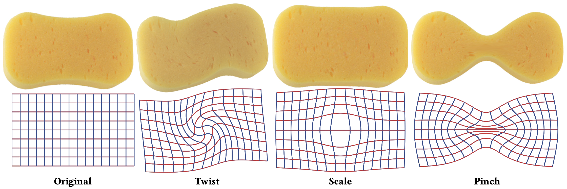 Fig. 5. Elastic Locally Affine Brushes: Given an input image (left), we compute a twisting (left-center), a scaling (center-right), and a pinching (right) deformation via a locally affine regularized Kelvinlet in 2D with Poisson ratio ν =0.4. Input image courtesy of Eftychios Sifakis.
Twisting: In the case of a skew-symmetric matrix, we can associate F to a vector q via the cross product matrix, i.e., $F \equiv[q]_{\times}$ where $[\boldsymbol{q}]_{\times} \boldsymbol{r}=\boldsymbol{q} \times \boldsymbol{r}$, then (14) simplifies to a twist deformation
``` iheartla
`$\boldsymbol{t}_ε$`(`$\boldsymbol{r}$`) = -a(1/`$r_ε$`³ + 3ε²/(2`$r_ε$`⁵) ) `$\boldsymbol{F}$``$\boldsymbol{r}$` where `$\boldsymbol{r}$` ∈ ℝ^3
```
By analyzing the deformation gradient of (15) (see supplemental material), one can verify that its symmetric part (the strain tensor) is trivial for any $\boldsymbol{r}$. Consequently, this displacement field has zero divergence (i.e., $\left.\nabla \cdot \boldsymbol{t}_ε(\boldsymbol{r})=0\right)$ ) and defines a volume preserving deformation, independent of the Poisson ratio ν. Instead, its curl is non-zero and can be used to relate the vector $\boldsymbol{q}$ to the vorticity $\bar{\omega}$ at $x_{0}$ via the linear constraint $\nabla \times t_ε(0)=\bar{\omega}$.
Scaling: Another type of locally affine regularized Kelvinlet can be generated by a force matrix of the form $F=s I$, where s is a scalar. In this case, (14) reduces to a scaling deformation
``` iheartla
`$\boldsymbol{s}_ε$`(`$\boldsymbol{r}$`) = (2b-a)(1/`$r_ε$`³ + 3ε²/(2`$r_ε$`⁵))(s`$\boldsymbol{r}$`) where `$\boldsymbol{r}$` ∈ ℝ^3
where
s ∈ ℝ
```
where positive values of $s$ represent contractions, and negative values determine dilations. Notice that we have $\boldsymbol{s}_ε ( \boldsymbol{r} ) = 0 $ for incompressible elastic materials, since $ν = 1/2$ implies $a = 2 b$ .
Pinching: The last type of locally affine regularized Kelvinlet is constructed based on a symmetric force matrix F with zero trace (in a total of 5 DoFs), and it generates displacements of the form
``` iheartla
`$\boldsymbol{p}_ε$`(`$\boldsymbol{r}$`) = (2b-a)/`$r_ε$`³ `$\boldsymbol{F}$``$\boldsymbol{r}$` - 3/(2`$r_ε$`⁵)(2b(`$\boldsymbol{r}$`ᵀ`$\boldsymbol{F}$``$\boldsymbol{r}$`)I_3+aε²`$\boldsymbol{F}$`)`$\boldsymbol{r}$` where `$\boldsymbol{r}$` ∈ ℝ^3
where
`$\boldsymbol{F}$` ∈ ℝ^(3×3): force matrix
`$r_ε$` ∈ ℝ
a ∈ ℝ : coefficient
b ∈ ℝ : coefficient
ε ∈ ℝ : the radial scale
```
To geometrically characterize this deformation, we computed the displacement gradient ∇pε at x0, and observed that the resulting matrix is also symmetric with zero trace. This indicates that the deformation generated by pε (r ) compensates infinitesimal stretching in one direction by contractions in the other directions, thus resembling a physical pinching interaction.
Multi-scale extrapolation: Since our affine brushes are based on the derivative of (6), the extrapolation scheme described in Section 5 applies to these displacement fields with no modification. We can then combine locally affine regularized Kelvinlets linearly and generate new matrix-driven solutions of linear elasticity with arbitrarily fast far-field decay. In particular, we obtain bi-scale and tri-scale brushes with $O\left(1 / r^{4}\right)$ and $O\left(1 / r^{6}\right)$ falloffs, respectively, while the single-scale case has an $O\left(1 / r^{2}\right)$ decay.
# CONSTRAINED DEFORMATIONS
By exploiting the linearity of (2), regularized Kelvinlets and variants can be superposed to form new solutions of linear elasticity. These compound brushes are of particular interest for designing deformations with pointwise contraints. Since regularized Kelvinlets are linear in terms of force vectors f and matrices F , these constrained deformations can be efficiently computed based on user-prescribed displacements and gradients. In this section, we describe some examples of constrained deformations.
Displacement Constraints: Previously we assigned the brush tip displacement u and solved analytically for the necessary force vector f in (7). We can replicate this constraint numerically for a list of brushes. To this end, we consider n regularized Kelvinlets placed at $\left\{x_{1}, \ldots, x_{n}\right\}$ and impose n displacement constraints $\left\{\overline{\boldsymbol{u}}_{1}, \ldots, \overline{\boldsymbol{u}}_{n}\right\}$, one for each brush center xi . By superposition, these brushes define a solution to (2) of the form
$$
\boldsymbol{u}(\boldsymbol{x})=\sum_{i=1}^{n} \mathcal{K}_{ε_{i}}\left(\boldsymbol{x}-\boldsymbol{x}_{i}\right) \boldsymbol{f}_{i}
$$
where $ε_i$ and $\boldsymbol{f}_{i}$ indicate the radial scale and the force vector for the i-th brush, respectively. The displacement constraints u and force vectors f are thus related by the linear system u = K f , where the 3n×3n matrix K has the contribution Kεi (xj − xi ) of every i-th brush to every j-th brush center.
An usual scenario for this constrained deformation is when we pin down zero displacement to n − 1 locations, and keep the n-th brush “live” for interactive sculpting. Given a tip displacement un updated every user edit, we can efficiently compute the force vectors f by exploiting the block structure of the linear system
$$
\left[\begin{array}{c}
0 \\
\bar{u}_{n}
\end{array}\right]=\left[\begin{array}{ll}
K_{p p} & K_{p n} \\
K_{n p} & K_{n n}
\end{array}\right]\left[\begin{array}{l}
f_{p} \\
f_{n}
\end{array}\right]
$$
where the subscript p indicates values for the n−1 pinned brushes, and n denotes the active brush. Observe that the block Kpp is a nonsymmetric matrix that relates the n−1 pinned brushes to themselves, but it is independent of the n-th brush. Therefore, we can cache the LU factorization of Kpp and solve for f rapidly at every user interaction via the Schur complement [@cottle1974manifestations], which then requires a simple 3×3 solve. Figure 6 (center-right) displays a result with displacement constraints used in a 3D editing session.
Gradient Constraints: We can also constrain the gradients of our deformations by employing locally affine regularized Kelvinlets in our compound displacement u(x). By doing so, the force matrix F can be used to precisely control the 9 DoFs of the deformation gradient via the linear constraint G(xi)=I +∇u(xi)atabrushcenter xi . This leads to the aggregated displacement field
$$
\boldsymbol{u}(\boldsymbol{x})=\sum_{i=1}^{n} \mathcal{A}_{ε_{i}}\left(\boldsymbol{x}-\boldsymbol{x}_{i}\right) \overrightarrow{\boldsymbol{F}}_{i}
$$
More specialized gradient control can be further achieved via individual twist, scale, and pinch brushes (Section 6). For instance, a pointwise vorticity constraint ∇×u can be enforced based on the 3 DoFs of the vector q in a twist brush, while the single parameter s of a scale brush can determine a divergence constraint ∇·u. We can also employ a pinch brush to control the infinitesimal stretches in two directions of a rotated frame, for a total of 5 DoFs. Note that the third infinitesimal strecth is induced by the first two values, since a pinch brush has a traceless gradient. Similar to the displacement case, these gradient constraints relate to their respective force parameters (F, q, or s) through a single linear system. As before, a Schur complement approach can be employed to speedup solve times when sculpting with fixed constraints. In Figure 6 (right), pointwise gradient constraints were used to ensure rigid deformations in selected regions of the eyeballs.
Symmetrized Deformations: A common feature in sculpting tools is the ability to symmetrize deformations by mirroring a brush operation across a user-specified plane. This is performed by replicating the brush at x0 to its image point x1 =c+M(x0−c), where M=I−2nnt indicatesthereflectionmatrixofaplanepassingthrough a base point c and with a normal vector n. The first case of symmetrized physically based deformation consists of copying a regularized Kelvinlet uε (r) of force vector f0 from x0 to x1, while keeping its radius ε but reflecting its force vector to f1 =M f0. The resulting deformation is then written as
Fig. 5. Elastic Locally Affine Brushes: Given an input image (left), we compute a twisting (left-center), a scaling (center-right), and a pinching (right) deformation via a locally affine regularized Kelvinlet in 2D with Poisson ratio ν =0.4. Input image courtesy of Eftychios Sifakis.
Twisting: In the case of a skew-symmetric matrix, we can associate F to a vector q via the cross product matrix, i.e., $F \equiv[q]_{\times}$ where $[\boldsymbol{q}]_{\times} \boldsymbol{r}=\boldsymbol{q} \times \boldsymbol{r}$, then (14) simplifies to a twist deformation
``` iheartla
`$\boldsymbol{t}_ε$`(`$\boldsymbol{r}$`) = -a(1/`$r_ε$`³ + 3ε²/(2`$r_ε$`⁵) ) `$\boldsymbol{F}$``$\boldsymbol{r}$` where `$\boldsymbol{r}$` ∈ ℝ^3
```
By analyzing the deformation gradient of (15) (see supplemental material), one can verify that its symmetric part (the strain tensor) is trivial for any $\boldsymbol{r}$. Consequently, this displacement field has zero divergence (i.e., $\left.\nabla \cdot \boldsymbol{t}_ε(\boldsymbol{r})=0\right)$ ) and defines a volume preserving deformation, independent of the Poisson ratio ν. Instead, its curl is non-zero and can be used to relate the vector $\boldsymbol{q}$ to the vorticity $\bar{\omega}$ at $x_{0}$ via the linear constraint $\nabla \times t_ε(0)=\bar{\omega}$.
Scaling: Another type of locally affine regularized Kelvinlet can be generated by a force matrix of the form $F=s I$, where s is a scalar. In this case, (14) reduces to a scaling deformation
``` iheartla
`$\boldsymbol{s}_ε$`(`$\boldsymbol{r}$`) = (2b-a)(1/`$r_ε$`³ + 3ε²/(2`$r_ε$`⁵))(s`$\boldsymbol{r}$`) where `$\boldsymbol{r}$` ∈ ℝ^3
where
s ∈ ℝ
```
where positive values of $s$ represent contractions, and negative values determine dilations. Notice that we have $\boldsymbol{s}_ε ( \boldsymbol{r} ) = 0 $ for incompressible elastic materials, since $ν = 1/2$ implies $a = 2 b$ .
Pinching: The last type of locally affine regularized Kelvinlet is constructed based on a symmetric force matrix F with zero trace (in a total of 5 DoFs), and it generates displacements of the form
``` iheartla
`$\boldsymbol{p}_ε$`(`$\boldsymbol{r}$`) = (2b-a)/`$r_ε$`³ `$\boldsymbol{F}$``$\boldsymbol{r}$` - 3/(2`$r_ε$`⁵)(2b(`$\boldsymbol{r}$`ᵀ`$\boldsymbol{F}$``$\boldsymbol{r}$`)I_3+aε²`$\boldsymbol{F}$`)`$\boldsymbol{r}$` where `$\boldsymbol{r}$` ∈ ℝ^3
where
`$\boldsymbol{F}$` ∈ ℝ^(3×3): force matrix
`$r_ε$` ∈ ℝ
a ∈ ℝ : coefficient
b ∈ ℝ : coefficient
ε ∈ ℝ : the radial scale
```
To geometrically characterize this deformation, we computed the displacement gradient ∇pε at x0, and observed that the resulting matrix is also symmetric with zero trace. This indicates that the deformation generated by pε (r ) compensates infinitesimal stretching in one direction by contractions in the other directions, thus resembling a physical pinching interaction.
Multi-scale extrapolation: Since our affine brushes are based on the derivative of (6), the extrapolation scheme described in Section 5 applies to these displacement fields with no modification. We can then combine locally affine regularized Kelvinlets linearly and generate new matrix-driven solutions of linear elasticity with arbitrarily fast far-field decay. In particular, we obtain bi-scale and tri-scale brushes with $O\left(1 / r^{4}\right)$ and $O\left(1 / r^{6}\right)$ falloffs, respectively, while the single-scale case has an $O\left(1 / r^{2}\right)$ decay.
# CONSTRAINED DEFORMATIONS
By exploiting the linearity of (2), regularized Kelvinlets and variants can be superposed to form new solutions of linear elasticity. These compound brushes are of particular interest for designing deformations with pointwise contraints. Since regularized Kelvinlets are linear in terms of force vectors f and matrices F , these constrained deformations can be efficiently computed based on user-prescribed displacements and gradients. In this section, we describe some examples of constrained deformations.
Displacement Constraints: Previously we assigned the brush tip displacement u and solved analytically for the necessary force vector f in (7). We can replicate this constraint numerically for a list of brushes. To this end, we consider n regularized Kelvinlets placed at $\left\{x_{1}, \ldots, x_{n}\right\}$ and impose n displacement constraints $\left\{\overline{\boldsymbol{u}}_{1}, \ldots, \overline{\boldsymbol{u}}_{n}\right\}$, one for each brush center xi . By superposition, these brushes define a solution to (2) of the form
$$
\boldsymbol{u}(\boldsymbol{x})=\sum_{i=1}^{n} \mathcal{K}_{ε_{i}}\left(\boldsymbol{x}-\boldsymbol{x}_{i}\right) \boldsymbol{f}_{i}
$$
where $ε_i$ and $\boldsymbol{f}_{i}$ indicate the radial scale and the force vector for the i-th brush, respectively. The displacement constraints u and force vectors f are thus related by the linear system u = K f , where the 3n×3n matrix K has the contribution Kεi (xj − xi ) of every i-th brush to every j-th brush center.
An usual scenario for this constrained deformation is when we pin down zero displacement to n − 1 locations, and keep the n-th brush “live” for interactive sculpting. Given a tip displacement un updated every user edit, we can efficiently compute the force vectors f by exploiting the block structure of the linear system
$$
\left[\begin{array}{c}
0 \\
\bar{u}_{n}
\end{array}\right]=\left[\begin{array}{ll}
K_{p p} & K_{p n} \\
K_{n p} & K_{n n}
\end{array}\right]\left[\begin{array}{l}
f_{p} \\
f_{n}
\end{array}\right]
$$
where the subscript p indicates values for the n−1 pinned brushes, and n denotes the active brush. Observe that the block Kpp is a nonsymmetric matrix that relates the n−1 pinned brushes to themselves, but it is independent of the n-th brush. Therefore, we can cache the LU factorization of Kpp and solve for f rapidly at every user interaction via the Schur complement [@cottle1974manifestations], which then requires a simple 3×3 solve. Figure 6 (center-right) displays a result with displacement constraints used in a 3D editing session.
Gradient Constraints: We can also constrain the gradients of our deformations by employing locally affine regularized Kelvinlets in our compound displacement u(x). By doing so, the force matrix F can be used to precisely control the 9 DoFs of the deformation gradient via the linear constraint G(xi)=I +∇u(xi)atabrushcenter xi . This leads to the aggregated displacement field
$$
\boldsymbol{u}(\boldsymbol{x})=\sum_{i=1}^{n} \mathcal{A}_{ε_{i}}\left(\boldsymbol{x}-\boldsymbol{x}_{i}\right) \overrightarrow{\boldsymbol{F}}_{i}
$$
More specialized gradient control can be further achieved via individual twist, scale, and pinch brushes (Section 6). For instance, a pointwise vorticity constraint ∇×u can be enforced based on the 3 DoFs of the vector q in a twist brush, while the single parameter s of a scale brush can determine a divergence constraint ∇·u. We can also employ a pinch brush to control the infinitesimal stretches in two directions of a rotated frame, for a total of 5 DoFs. Note that the third infinitesimal strecth is induced by the first two values, since a pinch brush has a traceless gradient. Similar to the displacement case, these gradient constraints relate to their respective force parameters (F, q, or s) through a single linear system. As before, a Schur complement approach can be employed to speedup solve times when sculpting with fixed constraints. In Figure 6 (right), pointwise gradient constraints were used to ensure rigid deformations in selected regions of the eyeballs.
Symmetrized Deformations: A common feature in sculpting tools is the ability to symmetrize deformations by mirroring a brush operation across a user-specified plane. This is performed by replicating the brush at x0 to its image point x1 =c+M(x0−c), where M=I−2nnt indicatesthereflectionmatrixofaplanepassingthrough a base point c and with a normal vector n. The first case of symmetrized physically based deformation consists of copying a regularized Kelvinlet uε (r) of force vector f0 from x0 to x1, while keeping its radius ε but reflecting its force vector to f1 =M f0. The resulting deformation is then written as
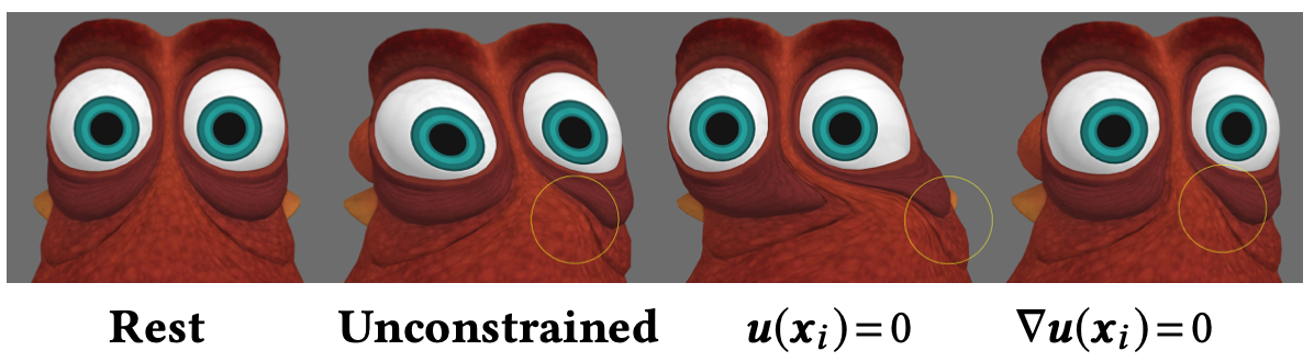 Fig. 6. Constraints: The deformation of an unconstrained regularized Kelvinlet distorts the eyeballs (left-center). The roundness of the irises and pupils can be restored by adding pointwise constraints. This is achieved by either pinning down zero displacements at these selected points (center-right), or enforcing locally rigid edits via gradient constraints (right). This example used a single 3D brush with ν = 1/2 and 160 constraints. ©Disney/Pixar
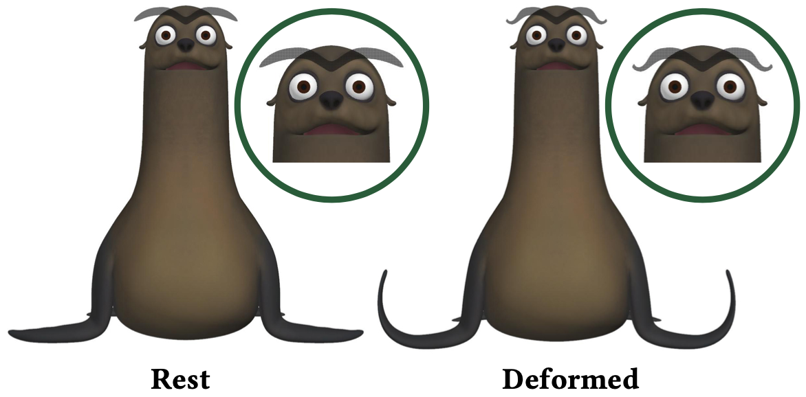 Fig. 7. Symmetrized edits: Regularized Kelvinlets also support symmetrized deformations. Here we show a symmetrized grab applied to the flippers, and a symmetrized twist sculpting the eyebrows of a sea lion. Both cases used a tri-scale brush in 3D with ν =1/2. ©Disney/Pixar
$$
\boldsymbol{u}(\boldsymbol{x})=\mathcal{K}_ε\left(\boldsymbol{x}-\boldsymbol{x}_{0}\right) f_{0}+\mathcal{K}_ε\left(\boldsymbol{x}-\boldsymbol{x}_{1}\right) f_{1}
$$
We show in the supplemental material that (21) satisfies the identity u(Mx)=M u(x) for any force vector f0 and at any evaluation point x, i.e., the displacement generated by (21) at the image of x is the reflection of the displacement at x. This also implies that the force vecor f0 can be computed from a given tip displacement u via a single constraint at x0.
Similarly, the symmetrization of locally affine brushes can be computed by mirroring the force matrix F0 to F1 =MF0M. The symmetrized displacement field is then
$$
u(x)=\mathscr{A}_ε\left(x-x_{0}\right) \vec{F}_{0}+\mathscr{A}_ε\left(x-x_{1}\right) \vec{F}_{1}
$$
As before, the force matrix F0 can be obtained in terms of a gradient constraint, if necessary. At last, we point out that multi-scale extrapolation applies to these formulations with no modification. Figure 7 shows symmetrized edits done by grab and twist brushes.
# 2D REGULARIZED KELVINLETS
We now discuss the construction of regularized Kelvinlets for an infinite elastic medium in R2. Besides image editing, these deformations are also suitable for volume sculpts restricted to the camera plane (Figure 8). In 2D, elastostatics is formulated using the same expressions for the energy (1) and for the equilibrium state (2) as in 3D, but now with differential operators ($\Delta$, ∇, ∇·) including only (x,y)-derivatives [@slaughter2012linearized]. This restriction introduces a new log term to the singular fundamental solutions [@phan1994microstructures], which makes our regularization scheme surpringsly more elaborated than the 3D case. As detailed next, we address the construction of 2D regularized Kelvinlets by considering a 2D body load as a 3D line force distribution passing through the brush center. This interpretation allows us to compute 2D solutions by integrating the associated 3D elastic responses through depth.
Fig. 7. Symmetrized edits: Regularized Kelvinlets also support symmetrized deformations. Here we show a symmetrized grab applied to the flippers, and a symmetrized twist sculpting the eyebrows of a sea lion. Both cases used a tri-scale brush in 3D with ν =1/2. ©Disney/Pixar
$$
\boldsymbol{u}(\boldsymbol{x})=\mathcal{K}_ε\left(\boldsymbol{x}-\boldsymbol{x}_{0}\right) f_{0}+\mathcal{K}_ε\left(\boldsymbol{x}-\boldsymbol{x}_{1}\right) f_{1}
$$
We show in the supplemental material that (21) satisfies the identity u(Mx)=M u(x) for any force vector f0 and at any evaluation point x, i.e., the displacement generated by (21) at the image of x is the reflection of the displacement at x. This also implies that the force vecor f0 can be computed from a given tip displacement u via a single constraint at x0.
Similarly, the symmetrization of locally affine brushes can be computed by mirroring the force matrix F0 to F1 =MF0M. The symmetrized displacement field is then
$$
u(x)=\mathscr{A}_ε\left(x-x_{0}\right) \vec{F}_{0}+\mathscr{A}_ε\left(x-x_{1}\right) \vec{F}_{1}
$$
As before, the force matrix F0 can be obtained in terms of a gradient constraint, if necessary. At last, we point out that multi-scale extrapolation applies to these formulations with no modification. Figure 7 shows symmetrized edits done by grab and twist brushes.
# 2D REGULARIZED KELVINLETS
We now discuss the construction of regularized Kelvinlets for an infinite elastic medium in R2. Besides image editing, these deformations are also suitable for volume sculpts restricted to the camera plane (Figure 8). In 2D, elastostatics is formulated using the same expressions for the energy (1) and for the equilibrium state (2) as in 3D, but now with differential operators ($\Delta$, ∇, ∇·) including only (x,y)-derivatives [@slaughter2012linearized]. This restriction introduces a new log term to the singular fundamental solutions [@phan1994microstructures], which makes our regularization scheme surpringsly more elaborated than the 3D case. As detailed next, we address the construction of 2D regularized Kelvinlets by considering a 2D body load as a 3D line force distribution passing through the brush center. This interpretation allows us to compute 2D solutions by integrating the associated 3D elastic responses through depth.
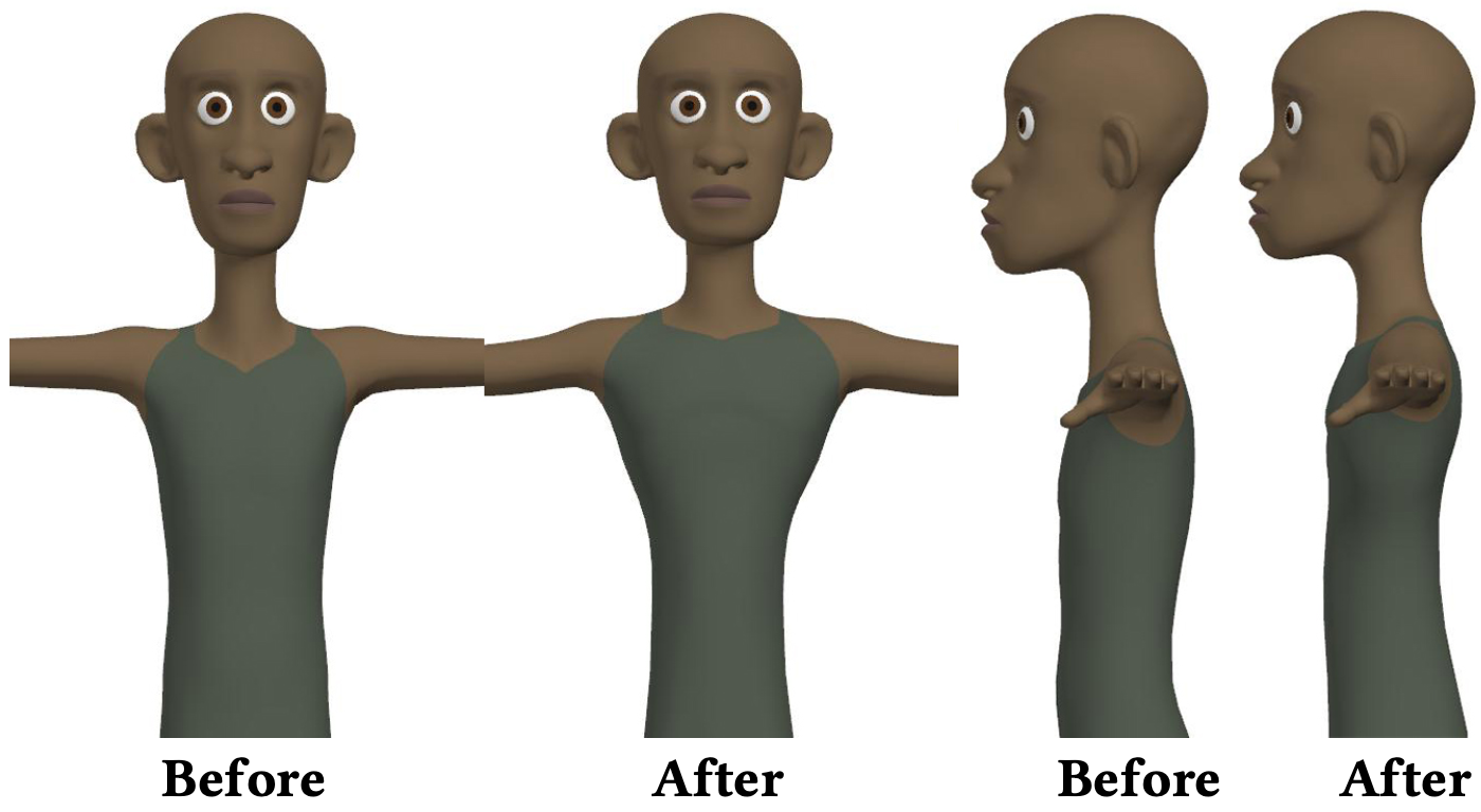 Fig. 8. Depth-preserving edits: A 2D regularized Kelvinlet with ν = 0.4 was used to bulge the chest of a human character (left), while maintaing the body thickness (right). In this case, the deformation was applied tangent to the camera plane, thus keeping the depth information intact. ©Disney/Pixar
Derivation: Hereafter we denote depth by the z-axis and use r to indicatethe2Drelativepositionvector(i.e.,r ≡[r,z]).Wereferto the 2D norm as r = ∥r∥, and to the regularized 2D distance as rε (so that rε2 =rε2+z2). We start by constructing a 2D force distribution that integrates the smoothed 3D density function ρε (r ) in (5) along the z-axis, producing
$$
\rho_ε(\mathfrak{r})=\int_{-\infty}^{+\infty} \rho_ε(\boldsymbol{r}) d z=\frac{2 ε^{2}}{\pi} \frac{1}{\mathfrak{r}_ε^{6}}
$$
With this density function, we can represent any 2D regularized Kelvinlet as the solution of (2) still in 3D, but now generated by aninfinitelineloadb(r)=fρε(r),where f hasitsz-componentset to zero. Due to symmetry, we can also show that the z-component of the 3D deformation generated by b(r) is zero. Therefore, the equation of elastostatics in 3D with load b(r) simplifies to its 2D counterpart with no z-derivatives. As a result, we can compute the 2D regularized Kelvinlet uε (r) by carefully integrating the (x,y) components of the 3D regularized Kelvinlet uε (r ),
$$
\left[\begin{array}{l}
u_ε^{x}(\mathfrak{r}) \\
u_ε^{y}(\mathfrak{r})
\end{array}\right]=\int_{-\infty}^{\infty}\left[\begin{array}{l}
u_ε^{x}(r) \\
u_ε^{y}(r)
\end{array}\right] d z
$$
which leads to the closed-form expression (see Appendix B)
$$
\boldsymbol{u}_ε(\mathfrak{r})=\left[2(b-a) \ln \left(\mathfrak{r}_ε\right) \boldsymbol{I}+2 b \frac{\mathfrak{r} \mathfrak{r}^{t}}{\mathfrak{r}_ε^{2}}+a \frac{ε^{2}}{\mathfrak{r}_ε^{2}} \boldsymbol{I}\right] \boldsymbol{f}
$$
We notice that (25) converges to the 2D singular Kelvinlets as ε approaches zero [@phan1994microstructures] and, in the incompressible limit (ν = 1/2), we obtain a 2D regularized Stokeslet. In contrast to [@cortez2001method], we employed a sharper 2D density function (given in (23)) that relates the regularization from 3D to 2D.
Multi-scale extrapolation: Compared to the 3D solutions, the regularized Kelvinlets in 2D introduce unbounded displacements as r → ∞, due to the presence of the log term, thus making them inappropriate for localized edits. Fortunately, the multi-scale extrapolation presented in Section 5 can be used to produce spatial falloffs. In fact, since 2D regularized Kelvinlets are integrated versions of the 3D displacements, the same multi-scale extrapolation rules previously stated for the 3D case work in 2D, and the observed far-field decay for bi-scale and tri-scale 2D brushes are O(1/r2) and O(1/r4), respectively.
Extension to affine loads: Following the same derivation from Section 6, we can also construct 2D versions of the locally affine regularized Kelvinlets, resulting in:
$$
\begin{aligned}
\widetilde{\boldsymbol{u}}_ε(\mathfrak{r})=&-2 a\left(\frac{1}{\mathfrak{r}_ε^{2}}+\frac{ε^{2}}{\mathfrak{r}_ε^{4}}\right) \boldsymbol{F r} \\
&+2 b\left[\frac{1}{\mathfrak{r}_ε^{2}}\left( \boldsymbol{F}+\boldsymbol{F}^{t}+\operatorname{tr}(\boldsymbol{F}) \boldsymbol{I}\right)-\frac{2}{\mathfrak{r}_ε^{4}}\left(\mathfrak{r}^{t} \boldsymbol{F} \mathfrak{r}\right) \boldsymbol{I}\right] \mathfrak{r},
\end{aligned}
$$
where F is now a 2×2 force matrix. Expressions for twisting (1-DoF), scaling (1-DoF) and pinching (2-DoF) can also be derived. We provide the list of closed-form solutions for 2D locally affine regularized Kelvinlets in the supplemental material.
# RESULTS
In this section, we detail our implementation and provide a series of experiments showcasing the performance and the visual quality of regularized Kelvinlets compared to existing sculpting tools. The accompanying video also includes several examples of editing sessions using our physically based brushes.
Implementation: We implemented regularized Kelvinlets and variants as a C++ plugin to the sculpting package of Pixar animation system (Presto). Once a brush type is selected, the brush center is assigned to the mouse click location, and the force parameters are set based on the mouse displacement. The user also has interactive control of the brush radius ε, the multi-scale mode (single, bi, or tri-scale), and the Poisson ratio ν. During a mouse event, we deform every selected point in the scene by moving them along the streamlines defined by the brush’s displacement field. This pointbased advection can be computed using any existing line integration method [@nielson1997scientific]. In our experiments, we employed a fourth-order Runge-Kutta method similar to [@von2006vector], but other integrators or substepping schemes can be easily incorporated. Notice that our deformation is evaluated at every selected point, including those outside the brush radius, because they may still have a non-zero displacement depending on the decay chosen for the brush. Therefore, the computational cost of our sculpts is linear on the number of selected points, in contrast to existing brushes that restrict the edits within the brush radius. In our implementation, we use multi-threading via TBB [@reinders2007intel], and observed performances averaging 57 frames per second on a 2.3 GHz Intel Xeon E5-2699 with 18 cores for scenes with 100k points. In the supplemental video, we also include a test with one million points, timing 18 ms per mouse drag. We expect even faster and more scalable running times by implementing regularized Kelvinlets in the GPU or as a geometry shader, which is feasible due to our closed-form analytical expressions.
Fig. 8. Depth-preserving edits: A 2D regularized Kelvinlet with ν = 0.4 was used to bulge the chest of a human character (left), while maintaing the body thickness (right). In this case, the deformation was applied tangent to the camera plane, thus keeping the depth information intact. ©Disney/Pixar
Derivation: Hereafter we denote depth by the z-axis and use r to indicatethe2Drelativepositionvector(i.e.,r ≡[r,z]).Wereferto the 2D norm as r = ∥r∥, and to the regularized 2D distance as rε (so that rε2 =rε2+z2). We start by constructing a 2D force distribution that integrates the smoothed 3D density function ρε (r ) in (5) along the z-axis, producing
$$
\rho_ε(\mathfrak{r})=\int_{-\infty}^{+\infty} \rho_ε(\boldsymbol{r}) d z=\frac{2 ε^{2}}{\pi} \frac{1}{\mathfrak{r}_ε^{6}}
$$
With this density function, we can represent any 2D regularized Kelvinlet as the solution of (2) still in 3D, but now generated by aninfinitelineloadb(r)=fρε(r),where f hasitsz-componentset to zero. Due to symmetry, we can also show that the z-component of the 3D deformation generated by b(r) is zero. Therefore, the equation of elastostatics in 3D with load b(r) simplifies to its 2D counterpart with no z-derivatives. As a result, we can compute the 2D regularized Kelvinlet uε (r) by carefully integrating the (x,y) components of the 3D regularized Kelvinlet uε (r ),
$$
\left[\begin{array}{l}
u_ε^{x}(\mathfrak{r}) \\
u_ε^{y}(\mathfrak{r})
\end{array}\right]=\int_{-\infty}^{\infty}\left[\begin{array}{l}
u_ε^{x}(r) \\
u_ε^{y}(r)
\end{array}\right] d z
$$
which leads to the closed-form expression (see Appendix B)
$$
\boldsymbol{u}_ε(\mathfrak{r})=\left[2(b-a) \ln \left(\mathfrak{r}_ε\right) \boldsymbol{I}+2 b \frac{\mathfrak{r} \mathfrak{r}^{t}}{\mathfrak{r}_ε^{2}}+a \frac{ε^{2}}{\mathfrak{r}_ε^{2}} \boldsymbol{I}\right] \boldsymbol{f}
$$
We notice that (25) converges to the 2D singular Kelvinlets as ε approaches zero [@phan1994microstructures] and, in the incompressible limit (ν = 1/2), we obtain a 2D regularized Stokeslet. In contrast to [@cortez2001method], we employed a sharper 2D density function (given in (23)) that relates the regularization from 3D to 2D.
Multi-scale extrapolation: Compared to the 3D solutions, the regularized Kelvinlets in 2D introduce unbounded displacements as r → ∞, due to the presence of the log term, thus making them inappropriate for localized edits. Fortunately, the multi-scale extrapolation presented in Section 5 can be used to produce spatial falloffs. In fact, since 2D regularized Kelvinlets are integrated versions of the 3D displacements, the same multi-scale extrapolation rules previously stated for the 3D case work in 2D, and the observed far-field decay for bi-scale and tri-scale 2D brushes are O(1/r2) and O(1/r4), respectively.
Extension to affine loads: Following the same derivation from Section 6, we can also construct 2D versions of the locally affine regularized Kelvinlets, resulting in:
$$
\begin{aligned}
\widetilde{\boldsymbol{u}}_ε(\mathfrak{r})=&-2 a\left(\frac{1}{\mathfrak{r}_ε^{2}}+\frac{ε^{2}}{\mathfrak{r}_ε^{4}}\right) \boldsymbol{F r} \\
&+2 b\left[\frac{1}{\mathfrak{r}_ε^{2}}\left( \boldsymbol{F}+\boldsymbol{F}^{t}+\operatorname{tr}(\boldsymbol{F}) \boldsymbol{I}\right)-\frac{2}{\mathfrak{r}_ε^{4}}\left(\mathfrak{r}^{t} \boldsymbol{F} \mathfrak{r}\right) \boldsymbol{I}\right] \mathfrak{r},
\end{aligned}
$$
where F is now a 2×2 force matrix. Expressions for twisting (1-DoF), scaling (1-DoF) and pinching (2-DoF) can also be derived. We provide the list of closed-form solutions for 2D locally affine regularized Kelvinlets in the supplemental material.
# RESULTS
In this section, we detail our implementation and provide a series of experiments showcasing the performance and the visual quality of regularized Kelvinlets compared to existing sculpting tools. The accompanying video also includes several examples of editing sessions using our physically based brushes.
Implementation: We implemented regularized Kelvinlets and variants as a C++ plugin to the sculpting package of Pixar animation system (Presto). Once a brush type is selected, the brush center is assigned to the mouse click location, and the force parameters are set based on the mouse displacement. The user also has interactive control of the brush radius ε, the multi-scale mode (single, bi, or tri-scale), and the Poisson ratio ν. During a mouse event, we deform every selected point in the scene by moving them along the streamlines defined by the brush’s displacement field. This pointbased advection can be computed using any existing line integration method [@nielson1997scientific]. In our experiments, we employed a fourth-order Runge-Kutta method similar to [@von2006vector], but other integrators or substepping schemes can be easily incorporated. Notice that our deformation is evaluated at every selected point, including those outside the brush radius, because they may still have a non-zero displacement depending on the decay chosen for the brush. Therefore, the computational cost of our sculpts is linear on the number of selected points, in contrast to existing brushes that restrict the edits within the brush radius. In our implementation, we use multi-threading via TBB [@reinders2007intel], and observed performances averaging 57 frames per second on a 2.3 GHz Intel Xeon E5-2699 with 18 cores for scenes with 100k points. In the supplemental video, we also include a test with one million points, timing 18 ms per mouse drag. We expect even faster and more scalable running times by implementing regularized Kelvinlets in the GPU or as a geometry shader, which is feasible due to our closed-form analytical expressions.
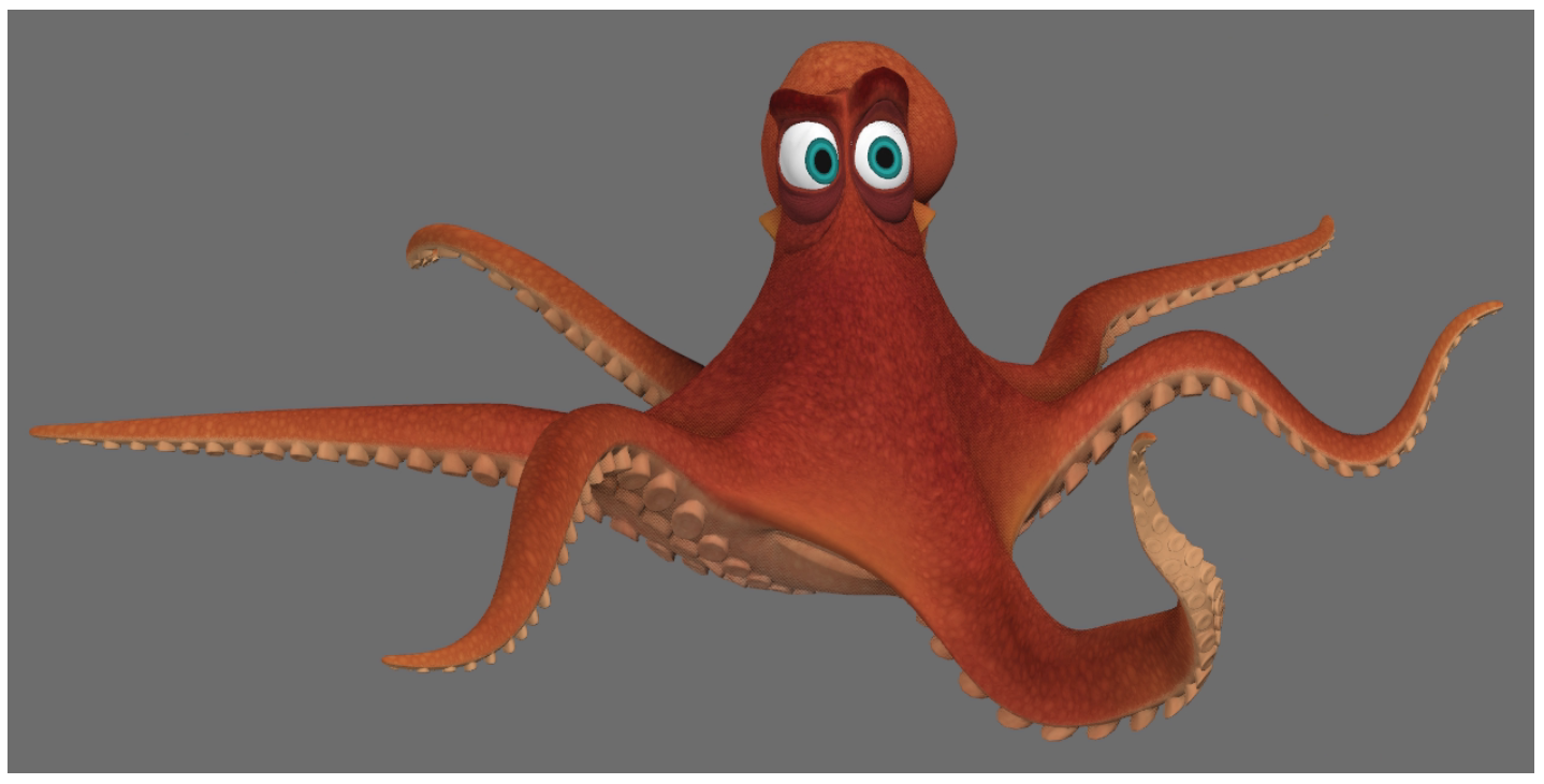 Fig. 9. Posing via sculpts: The final pose of a character sculpted by an artist using regularized Kelvinlet brushes exclusively. ©Disney/Pixar
Examples: Figures 2 and 5 illustrate the basic elastic deformations generated by displacement and affine loads, respectively. Figure 1 shows a gallery of facial expressions sculpted by an artist using combinations of our elastic brushes. Additionally, we include in Figure 9 a full-body deformed pose also sculpted by an artist via regularized Kelvinlets. We note that this model has multiple disconnected meshes, and our brush edits were applied to them simultaneously. In Figure 8, we used a 2D brush to bulge the chest of a character while preserving the body thicknesss. Figure 12 displays a sequence of volume edits with varying Poisson ratio. We demonstrate symmetrized grab and twist deformations in Figure 7. In Figure 6, we compare constrained deformations using displacement and gradient constraints. In this example, we employed the Schur complement approach described in Section 7 to precompute the constraint matrix only once during the mouse click, thus keeping the brush evaluation interactive. We point the reader to the supplemental video for additional examples and editing sessions.
Moving brushes: We can also modify the brush construction in order to support large deformations. So far our brush setup keeps its center stationary at the click location, and accumulates the force vector as the mouse moves. The resulting displacement may then introduce artifacts under large deformations, as expected from solutions of linear elasticity. Instead, by advecting the brush center throughout the course of the mouse edit, we can reset the force vector to the latest mouse shift and then reproduce within a single mouse click the deformation of a sequence of small clicks. Figure 10 shows an example that uses a moving brush to reduce distortion under large deformations. Note, however, that the deformation generated by a single click of a moving brush is path-dependent and may not restore the original shape as the mouse moves back to the click position, due to the accumulated displacements.
Fig. 9. Posing via sculpts: The final pose of a character sculpted by an artist using regularized Kelvinlet brushes exclusively. ©Disney/Pixar
Examples: Figures 2 and 5 illustrate the basic elastic deformations generated by displacement and affine loads, respectively. Figure 1 shows a gallery of facial expressions sculpted by an artist using combinations of our elastic brushes. Additionally, we include in Figure 9 a full-body deformed pose also sculpted by an artist via regularized Kelvinlets. We note that this model has multiple disconnected meshes, and our brush edits were applied to them simultaneously. In Figure 8, we used a 2D brush to bulge the chest of a character while preserving the body thicknesss. Figure 12 displays a sequence of volume edits with varying Poisson ratio. We demonstrate symmetrized grab and twist deformations in Figure 7. In Figure 6, we compare constrained deformations using displacement and gradient constraints. In this example, we employed the Schur complement approach described in Section 7 to precompute the constraint matrix only once during the mouse click, thus keeping the brush evaluation interactive. We point the reader to the supplemental video for additional examples and editing sessions.
Moving brushes: We can also modify the brush construction in order to support large deformations. So far our brush setup keeps its center stationary at the click location, and accumulates the force vector as the mouse moves. The resulting displacement may then introduce artifacts under large deformations, as expected from solutions of linear elasticity. Instead, by advecting the brush center throughout the course of the mouse edit, we can reset the force vector to the latest mouse shift and then reproduce within a single mouse click the deformation of a sequence of small clicks. Figure 10 shows an example that uses a moving brush to reduce distortion under large deformations. Note, however, that the deformation generated by a single click of a moving brush is path-dependent and may not restore the original shape as the mouse moves back to the click position, due to the accumulated displacements.
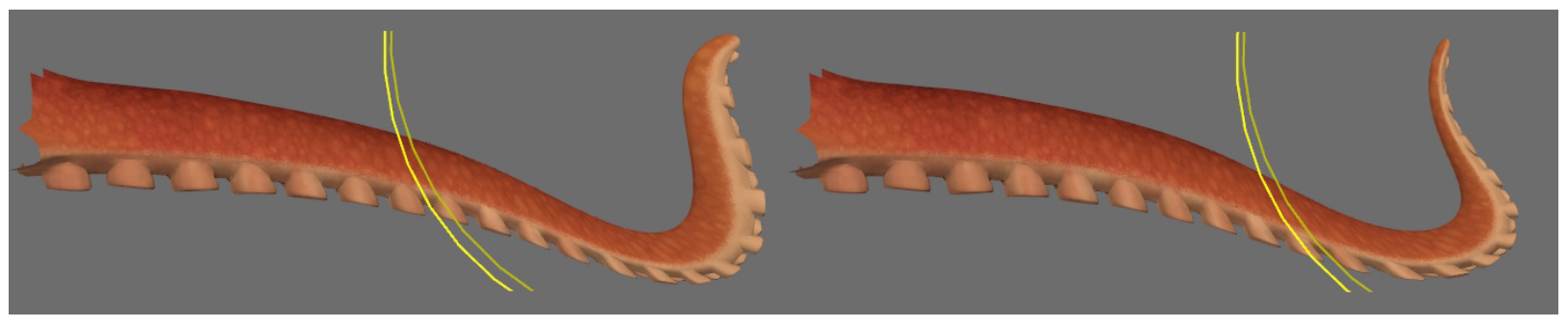 Fig. 10. Moving brush: Keeping the brush center stationary at the mouse click location leads to visual artifacts under large deformations (left). This distortion is alleviated by displacing the brush center during the mouse edit (right). ©Disney/Pixar
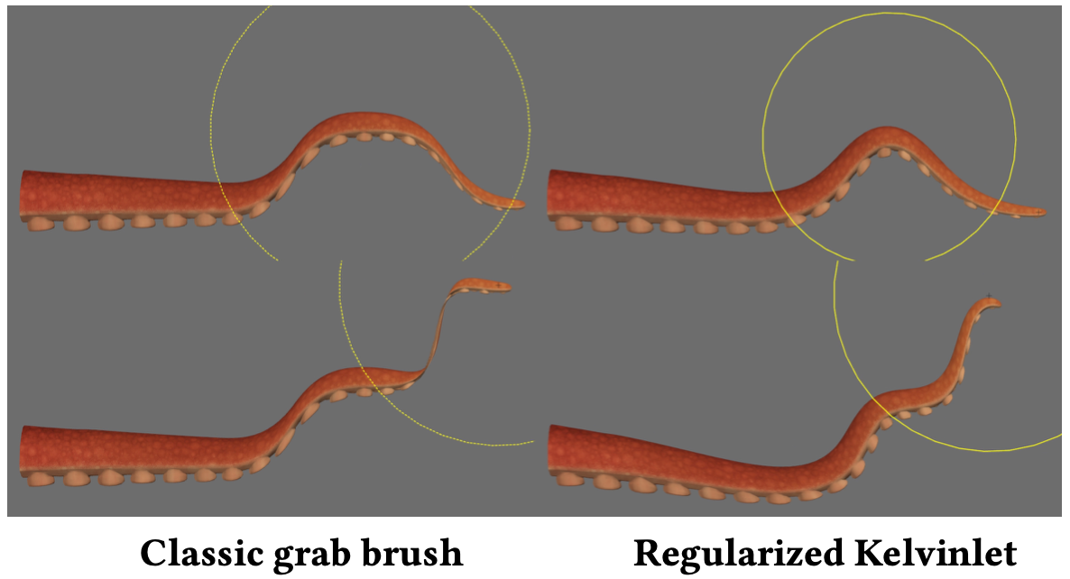 Fig. 11. Comparison: The left column shows results of two consecutive deformations using a grab brush with a Gaussian falloff. The right column shows the same two consecutive grabs now deformed by regularized Kelvinlets in 3D with Poisson ratio ν = 1/2. Notice how our physically based sculpting tool improves the local volume preservation. ©Disney/Pixar
Discussion: Figure 11 exhibits the deformation generated by a few clicks on a tentacle mesh using a (Maya-like) grab brush with a Gaussian falloff versus our 3D regularized Kelvinlet. This example illustrates the ability of our tool to capture broad volume deformations even with no knowledge of the surface structure, in contrast to traditional brushes that tend to collapse the volume. This result also suggests that our deformations could be used as an initial guess for iterative mesh-based deformers [@sorkine2007rigid] and simulators [@mcadams2011efficient], which can better capture mesh-dependent local features. While the physical values for the Poisson ratio lie within the range [0, 1/2] [@slaughter2012linearized], our method supports a broader spectrum of values. In particular, we show in Figure 2 that we can reproduce existing brushes with radial falloffs by setting ν = ±∞. We also notice that our twist deformation coincides to a swirling-sweeper brush with radial falloff [@angelidis2006swirling].
Limitations: The simplicity and speed of our approach come at the cost of several limitations. Foremost, since regularized Kelvinlets are solutions to the elasticity equations in an infinite continuum, they know nothing about the geometry they are used to deform. Consequently, they can not be used for accurate elastic analysis of solid shapes. Furthermore, surfaces deformed using regularized Kelvinlets move as if embedded in an infinite elastic continuum, thus disregarding any form of surface traction. Embedded deformations can also produce unintended and undesirable nonlocal interactions. For example, grabbing one tentacle can cause a second nearby tentacle to deform, even though these parts are far away geodesically. These issues motivate the use in the future of post-processing steps, such as surface-based masking, combined to our sculpting tools. We also point out that, while regularized Kelvinlets can produce smooth elastoplastic deformations, distorting discrete shapes may require dynamic remeshing in order to sufficiently resolve the flow with no visual artifacts (see, e.g., [@von2006vector]). We finally note that, even though we show results for posing deformable characters (Figure 9), our approach is primarily useful for relatively modest shape edits, and is not intended to replace articulated character rigs.
Fig. 11. Comparison: The left column shows results of two consecutive deformations using a grab brush with a Gaussian falloff. The right column shows the same two consecutive grabs now deformed by regularized Kelvinlets in 3D with Poisson ratio ν = 1/2. Notice how our physically based sculpting tool improves the local volume preservation. ©Disney/Pixar
Discussion: Figure 11 exhibits the deformation generated by a few clicks on a tentacle mesh using a (Maya-like) grab brush with a Gaussian falloff versus our 3D regularized Kelvinlet. This example illustrates the ability of our tool to capture broad volume deformations even with no knowledge of the surface structure, in contrast to traditional brushes that tend to collapse the volume. This result also suggests that our deformations could be used as an initial guess for iterative mesh-based deformers [@sorkine2007rigid] and simulators [@mcadams2011efficient], which can better capture mesh-dependent local features. While the physical values for the Poisson ratio lie within the range [0, 1/2] [@slaughter2012linearized], our method supports a broader spectrum of values. In particular, we show in Figure 2 that we can reproduce existing brushes with radial falloffs by setting ν = ±∞. We also notice that our twist deformation coincides to a swirling-sweeper brush with radial falloff [@angelidis2006swirling].
Limitations: The simplicity and speed of our approach come at the cost of several limitations. Foremost, since regularized Kelvinlets are solutions to the elasticity equations in an infinite continuum, they know nothing about the geometry they are used to deform. Consequently, they can not be used for accurate elastic analysis of solid shapes. Furthermore, surfaces deformed using regularized Kelvinlets move as if embedded in an infinite elastic continuum, thus disregarding any form of surface traction. Embedded deformations can also produce unintended and undesirable nonlocal interactions. For example, grabbing one tentacle can cause a second nearby tentacle to deform, even though these parts are far away geodesically. These issues motivate the use in the future of post-processing steps, such as surface-based masking, combined to our sculpting tools. We also point out that, while regularized Kelvinlets can produce smooth elastoplastic deformations, distorting discrete shapes may require dynamic remeshing in order to sufficiently resolve the flow with no visual artifacts (see, e.g., [@von2006vector]). We finally note that, even though we show results for posing deformable characters (Figure 9), our approach is primarily useful for relatively modest shape edits, and is not intended to replace articulated character rigs.
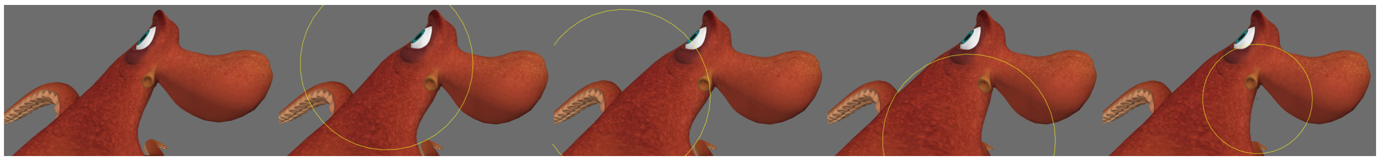 Fig.12. Volume adjustment: A series of one-click sculpts used for local volume adjustments. These deformations were computed using a regularized Kelvinlet in 2D with various values for the Poisson ratio. ©Disney/Pixar
# CONCLUSION
We have presented a family of deformation tools based on regularized fundamental solutions of linear elasticity for infinite media in 2D and 3D. Our method provides real-time feedback since it exploits closed-form analytical expressions and avoids the spatial discretization of elastic objects. This trade-off allows us to infuse “just enough” physical behavior into sculpting brushes to improve traditional grab, twist, pinch, and scale editing. We also addressed the problem of long-range interactions by introducing a multi-scale extrapolation scheme, and resolved various pointwise constraints using standard linear solves.
We believe this work opens up new possibilities for analytical methods to be used for real-time sculpting [@cani2006towards] and contact interactions [@pauly2004quasi]. We have introduced simple force primitives for brushes, but extensions with more general load distributions could be constructed for specialized purposes [@von2006vector]. Regularized fundamental solutions for a halfspace elastic continuum, such as the Boussinesq’s problem [PodioGuidugli and Favata 2014], and the method of images [@ainley2008method] are also of interest. Regularized Kelvinlets are also well-suited to kinesthetic haptic force and torque feedback, and to high-rate modeling applications in virtual and augmented reality.
# ACKNOWLEDGMENTS
We are grateful to Alonso Martinez and Kevin Singleton for generating the artistic examples in this work, and to Andrew Butts and Venkateswaran Krishna for their assistance with the Presto sculpting package. We also thank Michael Comet, Jeremie Talbot, Evan Bonifacio, and Dirk Van Gelder for discussions, and Tony DeRose, Theodore Kim, and Mathieu Desbrun for feedback on the manuscript. The image examples are courtesy of Mirela Ben-Chen (Figure 2) and Eftychios Sifakis (Figure 5).
Fig.12. Volume adjustment: A series of one-click sculpts used for local volume adjustments. These deformations were computed using a regularized Kelvinlet in 2D with various values for the Poisson ratio. ©Disney/Pixar
# CONCLUSION
We have presented a family of deformation tools based on regularized fundamental solutions of linear elasticity for infinite media in 2D and 3D. Our method provides real-time feedback since it exploits closed-form analytical expressions and avoids the spatial discretization of elastic objects. This trade-off allows us to infuse “just enough” physical behavior into sculpting brushes to improve traditional grab, twist, pinch, and scale editing. We also addressed the problem of long-range interactions by introducing a multi-scale extrapolation scheme, and resolved various pointwise constraints using standard linear solves.
We believe this work opens up new possibilities for analytical methods to be used for real-time sculpting [@cani2006towards] and contact interactions [@pauly2004quasi]. We have introduced simple force primitives for brushes, but extensions with more general load distributions could be constructed for specialized purposes [@von2006vector]. Regularized fundamental solutions for a halfspace elastic continuum, such as the Boussinesq’s problem [PodioGuidugli and Favata 2014], and the method of images [@ainley2008method] are also of interest. Regularized Kelvinlets are also well-suited to kinesthetic haptic force and torque feedback, and to high-rate modeling applications in virtual and augmented reality.
# ACKNOWLEDGMENTS
We are grateful to Alonso Martinez and Kevin Singleton for generating the artistic examples in this work, and to Andrew Butts and Venkateswaran Krishna for their assistance with the Presto sculpting package. We also thank Michael Comet, Jeremie Talbot, Evan Bonifacio, and Dirk Van Gelder for discussions, and Tony DeRose, Theodore Kim, and Mathieu Desbrun for feedback on the manuscript. The image examples are courtesy of Mirela Ben-Chen (Figure 2) and Eftychios Sifakis (Figure 5).