❤: soft
# SOFT COLOR SEGMENTATION
Our main objective in this paper is to decompose an image into multiple partially-transparent segments of homogeneous colors, i.e. soft color segments, which can then be used for various image manipulation tasks. Borrowing from image manipulation terminology, we will refer to such soft color segments simply as layers throughout this paper.
A crucial property of soft color segmentation is that overlaying all layers obtained from an image yields the original image itself so that editing individual layers is possible without degrading the original image. In mathematical terms, for a pixel $p$, we denote the opacity value as $α _i^p$ and the layer color in RGB as $\boldsymbol{u} ^p_i$ for the ith layer. and we want to satisfy the color constraint:
$$
\sum_{i} α _{i}^{p} \boldsymbol{u} _{i}^{p}=\boldsymbol{c}^{p} \quad \forall p
$$
where $c^p$ denotes the original color of the pixel. The total number of layers will be denoted by $N$.
We assume that the original input image is fully opaque, and thus require the opacity values over all layers to add up to unity, which we express as the alpha constraint:
$$
\sum_{i} α _{i}^{p}=1 \quad \forall p
$$
Finally, the permissible range for the alpha and color values are enforced by the box constraint:
$$
α _{i}^{p}, \boldsymbol{u} _{i}^{p} \in[0,1] \quad \forall i, p
$$
For convenience, we will drop the superscript p in the remainder of the paper and present our formulation at the pixel level, unless stated otherwise.
It should be noted that different representations for overlaying multiple layers exist. We use Equation 1, to which we refer as alpha-add representation, in our formulation which does not assume any particular ordering of the layers. This representation has also been used by Tai et al. [2007] and Chen et al. [2013] among others. In most commercial image editing software, however, the representation proposed by Porter and Duff [1984], referred in this paper as overlay representation, is used. The difference and conversion between the two representations are presented in the appendix.
Our algorithm for computing high-quality soft color segments can be described by three stages: color unmixing, matte regularization, and color refinement, which will be discussed in the remainder of this section.
Color Unmixing: An important property we want to achieve within each layer is color homogeneity: the colors present in a layer should be sufficiently similar. To this end, we associate each layer with a 3D normal distribution representing the spread of the layer colors in RGB space, and we refer to the set of $N$ distributions as the color model. Our novel technique for automatically extracting the color model for an image is discussed in detail in Section 5.
Given the color model, we propose the sparse color unmixing energy function in order to find a preliminary approximation to the layer colors and opacities:
``` iheartla
`$F_S$` = sum_i α_i D_i(`$\boldsymbol{u}$`_i) + σ((sum_i α_i)/(sum_i α_i^2) - 1)
where
D_i: ℝ^3 -> ℝ
`$\boldsymbol{u}$`_i: ℝ^3
σ: ℝ
α_i: ℝ
```
where the layer color cost $D _i( \boldsymbol{u} _i)$ is defined as the squared Mahalanobis distance of the layer color $\boldsymbol{u} _i$ to the layer distribution $N( \boldsymbol{u} _i, Σ_i)$, and $σ$ is the sparsity weight that is set to 10 in our implementation. The energy function in Equation 4 is minimized for all $α _i$ and $\boldsymbol{u} _i$ simultaneously while satisfying the constraints defined in Equations 1-3 using the original method of multipliers [Bertsekas 1982]. For each pixel, for the layer with best fitting distribution, we initialize the alpha value to 1 and the layer color ui to the pixel color. The rest of the layers are initialized to zero alpha value and the mean of their distributions as layer colors. The first term in Equation 4 favors layer colors that fit well with the corresponding distribution especially for layers with high alpha values, which is essential for getting homogeneous colors in each layer. The second term pushes the alpha values to be sparse, i.e. favors 0 or 1 alpha values.
The first term in Equation 4 appears as the color unmixing energy proposed by Aksoy et al. [2016] as a part of their system for green-screen keying. They do not include a sparsity term in their formulation, and this inherently results in favoring small alpha values, which results in many layers appearing in regions that should actually be opaque in a single layer. The reason is that a better-fitting layer color for the layer with alpha close to 1 (hence a lower color unmixing energy) becomes favorable by leaking small contributions from others (assigning small alpha values to multiple layers) with virtually no additional cost as the sample costs are multiplied with alpha values in the color unmixing energy. This decreases the compactness of the segmentation and, as a result, potentially creates visual artifacts when the layers are edited indepen- dently. Figure 2 shows such an example obtained through minimizing the color unmixing energy, where the alpha channel of the layer that captures the yellow road line is noisy on the asphalt region, even though the yellow of the road is not a part of the color of the asphalt. While these errors might seem insignificant at first, they result in unintended changes in the image when subjected to various layer manipulation operations such as contrast enhancement and color changes, as demonstrated in Figure 2.
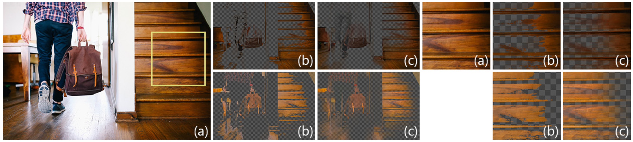
Fig. 3. Two layers corresponding to the dark (top) and light wood color in the original image (a) are shown before (b) and after (c) matte regularization and color refinement.
The sparsity term in Equation 4 is zero when one of the layers is fully opaque (and thus all other layers are fully transparent), and increases as the alpha values move away from zero or one. Another term for favoring matte sparsity has been proposed by Levin et al. [2008]:
$$
\sum_{i}\left| α _{i}\right|^{0.9}+\left|1- α _{i}\right|^{0.9}
$$
This cost is infinitely differentiable in the interval [0, 1]. Its infinite derivatives at $α _{i}=0^{+}$ and $α _{i}=1^{-}$ causes the alpha values to stay at these extremes in the optimization process we employ. In spectral matting, the behavior of this function is used to keep alpha values from taking values outside [0, 1]. In our case, as the box constraints are enforced during the optimization of the sparse color unmixing energy, the negative values our sparsity cost takes outside the interval do not affect our results adversely.
Matte Regularization: Sparse color unmixing is done independently for each pixel and there is no term ensuring spatial coherency. This may result in sudden changes in opacities that do not quite agree with the underlying image texture, as shown in Figure 3(b). Hence, spatial regularization of the opacity channels is necessary for ensuring smooth layers as in Figure 3(c). This issue also occurs frequently in sampling-based natural matting. The common practice for alpha regularization is using the matting Laplacian introduced by Levin et al. [2008] as the smoothness term and solve a linear system that also includes the spatially non-coherent alpha values, as proposed by Gastal and Oliveira [2010]. While this method is very effective in regularizing mattes, on the downside, it is computationally expensive and consumes a high amount of memory especially as the image resolution increases.
The guided filter proposed by He et al. [2013] provides an efficient way to filter any image using the texture information from a particular image, referred to as the guide image. The guided filter is an edge-aware filtering method that can make use of an image, the guide image, to extract the edge characteristics and filter a second image using the edge information from the guide image efficiently. They discuss the theoretical similarity between their filter and the matting Laplacian and show that getting satisfactory alpha mattes is possible through guided filtering when the original image is used as the guide image. While filtering the mattes with the guided filter only approximates the behavior of the matting Laplacian, we observed that this approximation provides sufficient quality for the mattes obtained through sparse color unmixing. For a 1 MP image, we use 60 as the filter radius and $10^{−4}$ as ε for the guided filter, as recommended by He et al. [2013] for matting, to regularize the alpha matte of each layer. As the resultant alpha values do not necessarily add up to 1, we normalize the sum of the alpha values for each pixel after filtering to get rid of small deviations from the alpha constraint. The filter radius is scaled according to the image resolution. Note that the layer colors are not affected by this filtering and they will be updated in the next step.
While enforcing spatial coherency on opacity channels is trivial using off-the-shelf filtering, dealing with its side effects is not straightforward. Obtaining spatially smooth results while avoiding disturbing color artifacts requires a second step that we discuss next.
Color Refinement: As the original alpha values are modified due to regularization, we can no longer guarantee that all pixels still satisfy the color constraint defined in Equation 1. Violating the color constraint in general severely limits the ability to use soft segments for image manipulation. For illustration, Figure 6 shows a pair of examples where KNN matting fails to satisfy the color constraint, which results in unintended color shifts in their results. To avoid such artifacts, we introduce a second energy minimization step, where we replace the alpha constraint defined in Equation 2 in the color unmixing formulation with the following term that forces the final alpha values to be as close as possible to the regularized alpha values:
$$
\sum_{i}\left( α _{i}-\hat{α }_{i}\right)^{2}=0
$$
where $\hat{α }_{i}$ represents the regularized alpha value of the $i^{th}$ layer. By running the energy minimization using this constraint, we recompute unmixed colors at all layers so that they satisfy the color constraint while retaining spatial coherency of the alpha channel. Note that since the alpha values are determined prior to this second optimization, the sparsity term in Equation 4 becomes irrelevant. Hence, we only employ the unmixing term of the energy in this step. For the optimization, we initialize the layer colors as the values found in the previous energy minimization step.
Finally, to summarize our color unmixing process: we first minimize the sparse color unmixing energy in Equation 4 for every pixel independently. We then regularize the alpha channels of the soft layers using the guided filter and refine the colors by running the energy minimization once again, this time augmented with the new alpha constraint defined in Equation 6. This way we achieve soft segments that satisfy the fundamental color, alpha, and box constraints, as well as the matte sparsity and spatial coherency requirements for high-quality soft-segmentation.
Note that the two energy minimization steps are computed independently for each pixel, and the guided filter can be implemented as a series of box filters. These properties make our algorithm easily parallelizable and highly scalable.